ML Interview Q Series: Analyzing EV Lifetime Differences Using Gaussian Probability Distributions

Browse all the Probability Interview Questions here.

34. Say that the lifetime of electric vehicles are modeled by a Gaussian distribution, with a certain mean and variance for each type. If you pick two different vehicle types at random, what is the probability their lifetimes differ by at most n units?

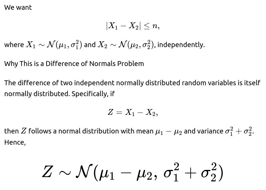
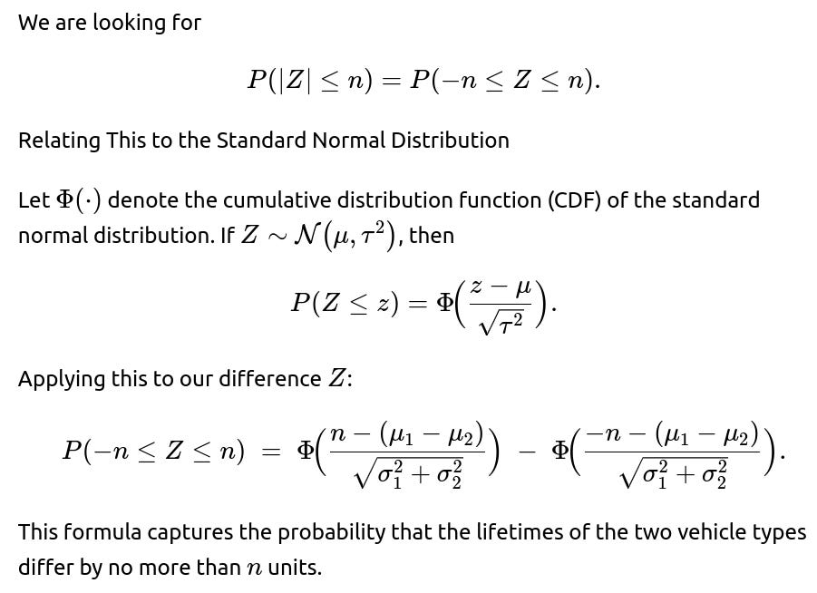
That is the most direct closed-form expression for the probability that the lifetimes differ by at most nn.

Example Code Snippet in Python

import numpy as np
from math import erf, sqrt

def probability_lifetimes_within_n(mu1, sigma1, mu2, sigma2, n):
    # mean and standard deviation of the difference
    mu_diff = mu1 - mu2
    sigma_diff = np.sqrt(sigma1**2 + sigma2**2)

    # Standardize the boundaries
    upper_z = (n - mu_diff) / sigma_diff
    lower_z = (-n - mu_diff) / sigma_diff

    # Use error function to get CDF for normal distribution
    # Equivalent to: Phi(z) = 0.5 * (1 + erf(z / sqrt(2)))
    def phi(z):
        return 0.5 * (1 + erf(z / np.sqrt(2)))

    prob = phi(upper_z) - phi(lower_z)
    return prob

# Example usage
mu1, sigma1 = 100, 10
mu2, sigma2 = 105, 12
n = 5

result = probability_lifetimes_within_n(mu1, sigma1, mu2, sigma2, n)
print("Probability they differ by at most n units:", result)

Practical Considerations

Occasionally, engineers might also want to incorporate more nuanced assumptions, such as non-independence between vehicle types (for instance, if they share certain battery components or have manufacturing processes in common). But in the standard approach, we treat them as independent.

What if the Two Vehicle Types Come From a Larger Pool With Different Probabilities?

What Happens if the Distributions Are Not Independent?

What Are Potential Edge Cases or Pitfalls?

One subtlety arises if the standard deviations differ significantly. For example, one vehicle type might have a lifetime distribution that is quite spread out (high variance) and another that is very precise (low variance). The difference distribution might be quite wide, making it less likely to remain within a narrow band nn.

Another potential pitfall is numerical stability. If n is extremely large or extremely small, one might run into floating-point issues when using the CDF of the normal distribution. Libraries like SciPy handle extreme values more gracefully than manual computations with the error function.

Example Follow-up Questions and Detailed Answers

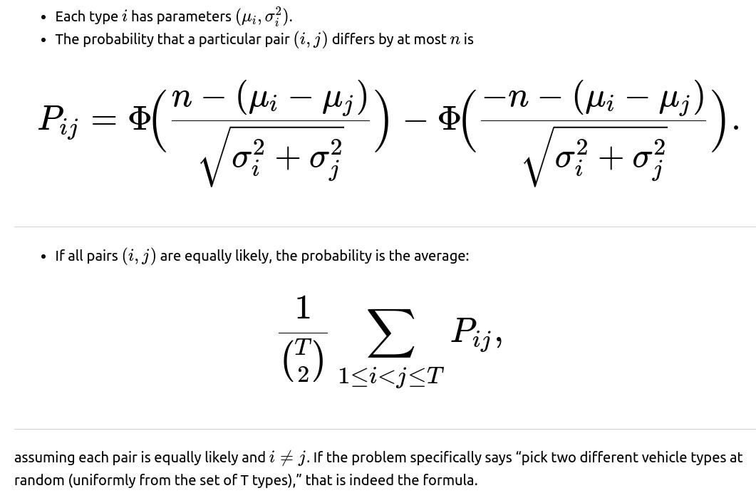
How can we extend this to more than two vehicle types to find the probability that any two randomly chosen vehicles differ by at most n?

You would average (or compute an expectation of) the probability that their lifetimes differ by at most n over all distinct pairs of vehicle types. If there are T types in total, index them by 1,2,…,T

What if we only have sample data for each type’s lifetime rather than known means and variances?

Can we approximate or bound this probability without computing normal CDF?

If lifetimes are not perfectly Gaussian, can we still use this approach?

Often, real-world lifetimes might not be strictly normal (e.g., they could be closer to a Weibull distribution or lognormal distribution). However, if the question states that we are “modeling by a Gaussian distribution,” that implies an assumption or approximation that it is normal enough. If the actual distribution deviates significantly from normal, the difference might not be exactly normal. Still, by the Central Limit Theorem or by engineering approximations, the normal model is often used as a practical tool, especially if the lifetime distribution is unimodal and not heavily skewed. In high-stakes engineering contexts, you might do deeper distributional fitting or reliability modeling that goes beyond a simple normal assumption.

If the means are very close but the variances are large, how does this affect the probability?

Could there be confusion with absolute difference vs. standard difference?

What if we want the distribution of the ratio instead of the difference?

Summary of Key Points

This formula is the essential result.

Below are additional follow-up questions

If the two vehicle types have very small sample sizes, how would we handle estimating their means and variances for this probability calculation?

When each type has only a small number of observed lifetime data points, statistical estimates for the mean and variance become less stable. In such cases:

• We would typically compute sample means and sample variances using the available data. For type (i), let:

  • (\hat{\mu}i = \frac{1}{N_i} \sum{k=1}^{N_i} x_{ik}), where (x_{ik}) are the observed lifetimes of type (i).

  • (\hat{\sigma}i^2 = \frac{1}{N_i - 1} \sum{k=1}^{N_i} \bigl(x_{ik} - \hat{\mu}_i\bigr)^2).

• Because (N_i) is small, confidence intervals for (\hat{\mu}_i) and (\hat{\sigma}_i^2) will be wide, and there is considerable uncertainty in these estimates. One might use:

  • T-distribution approaches for smaller sample sizes if normality is assumed (for the sample mean).

  • Adjusted or Bayesian estimators that incorporate prior information about typical battery lifetimes or known manufacturing constraints.

• Once we have an estimate (\hat{\mu}_i) and (\hat{\sigma}_i^2), we can still plug them into the same formula for the difference of normals. But we must note that the resulting probability is also an estimate with its own uncertainty. If one is concerned about risk (e.g., guaranteeing a certain probability), one might use statistical bounds such as the upper confidence bound on the difference distribution’s variance to be more conservative.

• A subtle, real-world pitfall is that with small (N_i), outliers heavily affect mean and variance. If a single vehicle in a test had a defective battery, it might severely distort (\hat{\mu}_i) or (\hat{\sigma}_i^2). Robust statistical methods (e.g., trimmed means, robust estimators) might be more appropriate to handle outliers.

What if there are significant non-stationarities over time, such as improvements in technology causing the distributions to shift?

If technology is rapidly improving, the mean lifetimes might not be static. For instance, a 2021 model might have a lower mean lifetime than a 2025 model of the “same” type due to battery chemistry enhancements. This leads to:

• Time-varying parameters: (\mu_i(t)) and (\sigma_i^2(t)). If we pick “type (i)” at random but that type has evolved over multiple manufacturing runs, the distribution might be a blend of sub-distributions.

• A potential solution is to stratify data by production batches or by year and model each generation of a vehicle type separately. Then, the question about picking “two different vehicle types at random” might become “two different vehicle types from the same era” or “two from potentially different eras.” The probability can shift significantly if we aggregate across multiple generations.

• A real-world pitfall is ignoring these technology shifts and combining all data into a single normal distribution. This can blur important differences in early vs. later production runs. Consequently, the actual probability that the lifetimes differ by at most (n) might be misrepresented if we don’t treat these differences carefully.

How would we factor in scenario-based constraints, such as usage patterns or climate conditions, that might alter the variance?

Vehicle lifetimes can depend heavily on external factors such as charging habits, climate, terrain, or average driving distance per day. If different vehicle types are tested under different conditions, the distributions might not be purely a property of “type” but also of “environment.” In practice:

• One approach is to condition on usage patterns. For each vehicle type (i), we define separate distributions (\mathcal{N}(\mu_{i,j}, \sigma_{i,j}^2)) for usage pattern (j). Then, the difference depends on picking vehicle type (i) under pattern (j) vs. vehicle type (k) under pattern (\ell). We would have: [ \huge X_{i,j} \sim \mathcal{N}(\mu_{i,j}, \sigma_{i,j}^2) ] and so [ \huge X_{k,\ell} \sim \mathcal{N}(\mu_{k,\ell}, \sigma_{k,\ell}^2), ] leading to a difference distribution with mean (\mu_{i,j} - \mu_{k,\ell}) and variance (\sigma_{i,j}^2 + \sigma_{k,\ell}^2).

• A real-world pitfall: Overlooking that one vehicle type might be predominantly used by frequent fast-chargers in a hot climate, while another type is used mostly in moderate climates with slow-charging behavior. Directly comparing their lifetime distributions might conflate type differences with usage environment differences.

If we have partial correlations between vehicle types due to shared battery suppliers, how does that influence the result?

When vehicle types share common components or suppliers, their lifetimes may not be truly independent. For instance, if both Type A and Type B use batteries from the same supplier, and that supplier’s production quality can fluctuate, there could be a positive correlation ((\rho > 0)) in their lifetimes. This alters the variance of the difference:

• For correlated normal variables (X_1) and (X_2) with correlation (\rho), [ \huge \mathrm{Var}(X_1 - X_2) = \sigma_1^2 + \sigma_2^2 - 2\rho , \sigma_1 \sigma_2. ]

• If (\rho) is positive and substantial, it reduces the variance of (X_1 - X_2). That means the difference distribution is narrower, which increases the probability that (|X_1 - X_2| \le n) (assuming (\mu_1\approx\mu_2)). On the other hand, if (\mu_1) is not close to (\mu_2), the correlation might not help as much because the mean shift still matters.

• A subtle pitfall is incorrectly assuming independence when there is correlation. This can lead to incorrectly inflating the difference variance. Practically, you might see an unexpectedly high observed rate of “similar lifetimes” if you ignore the correlation.

What if the means and variances are themselves random variables due to uncertainty in manufacturing, and we want a “distribution of distributions”?

In some advanced settings, engineers treat the parameters (\mu_i) and (\sigma_i^2) themselves as random because each production batch can vary. This is a hierarchical model perspective:

• At the top level, we have distributions over (\mu_i) and (\sigma_i^2).

• Conditional on (\mu_i) and (\sigma_i^2), lifetimes (X_{i}) follow (\mathcal{N}(\mu_i, \sigma_i^2)).

If we want the probability (\mathbb{P}(|X_i - X_j| \le n)) “averaged” over possible draws of parameters, we might do a Bayesian integral:

[

\huge \mathbb{E}_{\mu_i, \sigma_i^2, \mu_j, \sigma_j^2}\Bigl[ \mathbb{P}\bigl(|X_i - X_j| \le n ,\big|\mu_i, \sigma_i^2,\mu_j, \sigma_j^2\bigr)\Bigr]. ]

• This is more computationally intense, as it involves integrating over posterior distributions of the means and variances. Tools like Markov Chain Monte Carlo can be used.

• Pitfalls include model mis-specification (e.g., assuming prior distributions that don’t reflect real manufacturing variability) and the complexity of implementing a hierarchical Bayesian model. But in some R&D scenarios with limited data, it offers a more nuanced representation of uncertainty.

Could the presence of outliers or heavy-tailed distributions compromise the normal assumption in a way that significantly affects the difference distribution?

Yes, real-world battery lifetimes can exhibit heavier tails than a normal distribution—for instance, some batteries might fail prematurely (far-left tail) or occasionally last much longer than average (far-right tail). If the distribution is heavy-tailed (e.g., more akin to a Student’s t-distribution or a lognormal with large variance), then:

• The difference of two such heavy-tailed variables may not be well-approximated by a normal for smaller sample sizes. The central limit theorem eventually pushes things toward normal, but in practical sample sizes, tails can still be heavier, leading to more frequent extreme differences.

• The probability (\mathbb{P}(|X_1 - X_2| \le n)) might differ substantially from what the normal formula predicts if those tails matter. In particular, the presence of outliers could inflate the empirical variance, or the distribution might show skewness that the normal assumption doesn’t capture.

• A real-world pitfall: Underestimating the probability of large differences. The normal-based calculation might say that large differences are unlikely, but heavy-tailed reality might produce them more often than expected.

How would we handle discrete or zero-truncated data (e.g., if certain types can’t have lifetimes below a threshold)?

In some scenarios, you can’t have negative or very low lifetimes, especially if the manufacturer sets a minimum standard or if the measurement is discretized (e.g., only integer weeks of service are recorded). Then the normal assumption may not strictly hold near the boundary. Possible approaches:

• A truncated normal model: (\mathcal{N}(\mu_i, \sigma_i^2)) restricted to values above some lower bound (or possibly above zero). The difference distribution is then more complex to derive analytically, because each (X_i) is truncated in a different range. You typically rely on specialized software to compute (\mathbb{P}(|X_1 - X_2| \le n)).

• A discrete approximation or direct empirical approach: If the data are only integer lifetimes, you might estimate the probability distribution directly from the empirical frequencies and then convolve them to get the difference distribution. This might be more transparent but can require more data.

• Real-world pitfall: If you ignore the truncation and apply a standard normal formula, you might incorrectly permit negative lifetimes or produce an invalid probability for large differences. The discrepancy might be minimal if the truncation is well below the typical operating range, but if the truncation is near the mean, it can heavily distort results.

If we use the difference-of-normals approach but suspect multiple modes (e.g., a bimodal distribution), how would we adapt?

If a single vehicle type is actually composed of subpopulations with distinct means (for instance, different battery suppliers for the same model leading to two distinct lifetime “clusters”), that distribution may be closer to a mixture of Gaussians rather than a single Gaussian. For instance, for vehicle type (i), we might have:

[

\huge X_i \sim \pi ,\mathcal{N}(\mu_{i,1}, \sigma_{i,1}^2) + (1-\pi),\mathcal{N}(\mu_{i,2}, \sigma_{i,2}^2). ]

Then the difference between two mixture distributions is itself a mixture of difference-of-Gaussians. To get (\mathbb{P}(|X_1 - X_2| \le n)), you sum over all pairwise components:

[

\huge \mathbb{P}(|X_1 - X_2| \le n) = \sum_{a,b} \bigl(\pi_a \pi_b\bigr) , \mathbb{P}\bigl(|Y_{a,b}| \le n\bigr), ] where (Y_{a,b}) is the difference of the specific Gaussian components. Each difference (\mathcal{N}(\mu_{1,a} - \mu_{2,b},, \sigma_{1,a}^2 + \sigma_{2,b}^2)). Then you weight by the mixture probabilities (\pi_a\pi_b).

• Real-world pitfall: If we treat a bimodal distribution as unimodal, we might incorrectly flatten the distribution. This can incorrectly increase or decrease the probability of being within (n). The mismatch can be especially large if the two modes are separated by more than a few standard deviations.

If we want to optimize over (n) (e.g., find the smallest (n) that guarantees a 90% probability), how would we proceed?

Sometimes, instead of a fixed (n), you want to determine the threshold (n) that ensures (\mathbb{P}(|X_1 - X_2| \le n) \geq 0.90). The question becomes: Solve for (n) in

[

\huge \Phi\Bigl(\frac{n - (\mu_1 - \mu_2)}{\sqrt{\sigma_1^2 + \sigma_2^2}}\Bigr)

• \Phi\Bigl(\frac{-n - (\mu_1 - \mu_2)}{\sqrt{\sigma_1^2 + \sigma_2^2}}\Bigr) = 0.90. ]

• One approach is a simple numerical search (e.g., bisection or Newton’s method).

• A subtlety is that if (\mu_1) and (\mu_2) differ significantly, no small (n) can achieve a 90% probability. In that case, the solution for (n) might be quite large.

• A practical scenario: A company might want to guarantee that “the difference in lifetimes between Model A and Model B will be within a certain threshold for 90% of their production.” They would solve for that threshold using data for (\mu_A, \sigma_A, \mu_B, \sigma_B).

If the random draws of two different vehicle types are not equally probable (some are more commonly produced), how does it change the interpretation?

If certain types dominate production volume, picking two vehicles at random from the total production might heavily favor those high-volume types. However, the original question might be about picking vehicle “types” themselves uniformly, which is different. In real practice:

• If we literally pick “two vehicles from the fleet” at random, more common types are overrepresented. This changes the probability distribution for (\mu_i) and (\sigma_i). We might have a higher chance of picking types with large production volume.

• A pitfall is conflating “picking two types at random from a list of available types” with “picking two vehicles at random from the entire fleet.” These can give different probabilities of lifetime differences, because the latter approach is weighted by real-world production proportions.

What challenges arise if the measured lifetime is censored (e.g., some vehicles are still on the road so their end-of-life is unknown)?

In many reliability studies, we might only know that certain vehicles “have not failed up to now,” so their exact lifetime remains unknown. This is right-censoring. Handling censoring properly:

• Requires survival analysis techniques like maximum likelihood estimation under the assumption of a particular parametric distribution (e.g., normal, lognormal, Weibull).

• The estimated (\hat{\mu}_i) and (\hat{\sigma}_i^2) for each type must incorporate censored data. Naively ignoring the censoring by treating those vehicles as if they had lifetimes equal to the time so far can bias downward the estimated mean lifetime.

• If a large proportion of data is censored, the confidence in (\hat{\mu}_i) and (\hat{\sigma}_i^2) is reduced, and the final probability (\mathbb{P}(|X_1 - X_2| \le n)) has higher uncertainty. Detailed modeling or iterative numeric methods (like expectation-maximization or specialized survival analysis software) may be needed.

How might we validate or sanity-check the resulting probability in real-world pilot tests?

Even with a well-grounded model, it’s prudent to verify that the theoretical probability (\mathbb{P}(|X_1 - X_2| \le n)) aligns with empirical observations:

• One approach is to collect a sample of vehicles from Type 1 and Type 2, measure their actual lifetimes (or at least approximate them), and compute how often (|\text{lifetime}_1 - \text{lifetime}_2| \le n). Compare this empirical proportion to the model’s predicted probability.

• If there’s a discrepancy, investigate possible causes:

  • Parameter misestimation (means or variances are off),

  • Normal assumption being invalid,

  • Correlation or mixture effects,

  • Unrepresentative sampling in the pilot test.

• Such validation helps catch systematic biases. For example, if your model systematically overestimates the probability (predicts that the difference is smaller than it actually is), you might discover unmodeled heavy tails or wide usage variations.

How do small changes in the parameters (like a slight shift in mean or variance) affect this probability in a boundary scenario?

In boundary scenarios—where (\mu_1\approx \mu_2) or (\sigma_1^2 + \sigma_2^2) is quite small—tiny changes can significantly impact (\mathbb{P}(|X_1 - X_2| \le n)). Specifically:

• If (\mu_1\approx \mu_2) and (\sigma_1^2 + \sigma_2^2) is small, the difference distribution is narrowly centered around 0. Even a small shift in (\mu_1 - \mu_2) can push the difference outside the range ([-n, +n]), dramatically reducing the probability.

• This can happen in real production lines where a small manufacturing change slightly alters battery longevity. If the original design yielded nearly identical lifetimes, a marginal shift might yield a surprising jump (up or down) in the fraction of vehicles whose difference is within (n).

• Practically, companies might track such sensitivity by partial derivatives or by direct “what if” scenario testing: “If (\mu_1) increases by 1%, how does that affect the probability?”

How does sampling variability in measuring (\mu_1, \sigma_1^2, \mu_2, \sigma_2^2) translate into a confidence interval on (\mathbb{P}(|X_1 - X_2| \le n))?

When each parameter is estimated from data, we can propagate the uncertainties to get a confidence interval on the final probability. For instance:

• Suppose we have approximate standard errors for (\hat{\mu}_1), (\hat{\sigma}_1^2), (\hat{\mu}_2), and (\hat{\sigma}_2^2). We could use the delta method (a statistical tool) to approximate the variance of the function: [ \huge f(\hat{\mu}_1, \hat{\sigma}_1^2, \hat{\mu}_2, \hat{\sigma}_2^2) = \mathbb{P}(|X_1 - X_2| \le n). ]

• Alternatively, a bootstrap approach can be used: repeatedly resample from the observed data for each type, re-estimate (\mu_i) and (\sigma_i^2), and recalculate the probability. This yields an empirical distribution of (\mathbb{P}(|X_1 - X_2| \le n)) values, from which a confidence interval can be derived.

• A key pitfall is ignoring the sampling variability. One might report only a point estimate for (\mathbb{P}(|X_1 - X_2| \le n)). In an interview scenario, acknowledging the existence of a confidence interval (or Bayesian credible interval) shows deeper understanding of real-world data analysis.

Are there any special considerations if we do pairwise comparisons among multiple vehicle types and then want to control for multiple hypotheses?

When comparing more than two types—say, a large set of vehicles with different means and variances—you might do pairwise probability calculations (\mathbb{P}(|X_i - X_j| \le n)) for many pairs ((i, j)). In a hypothesis-testing framework, each comparison could be considered a “null hypothesis” or part of a family of tests:

• If you want to declare “vehicle types (i) and (j) are within (n) of each other in lifetime,” and do so for many pairs, you might face issues of multiple testing. Standard corrections (Bonferroni, Benjamini–Hochberg, etc.) may be required to control the family-wise error rate or false discovery rate.

• In a purely probabilistic sense (not hypothesis testing), it might just be a large matrix of probabilities. But once you interpret these probabilities as statistically significant statements, the usual multiple-comparison problem arises.

• A practical pitfall is to conduct many pairwise comparisons and over-interpret them. This can lead to spurious claims about differences or similarities, especially if the underlying data is noisy.