
ML Interview Q Series: Analyzing Expected Downtime for Parallel Systems with Exponential Lifetimes and Periodic Maintenance.

Browse all the Probability Interview Questions here.
An unreliable electronic system has two components hooked up in parallel. The lifetimes X and Y of the two components have the joint density f(x,y) = e^(-(x + y)) for x,y ≥ 0. The system goes down when both components have failed. The system is inspected every T time units, and at inspection any failed unit is replaced.
(a) What is the probability that the system goes down between two inspections?
(b) What is the expected amount of time the system is down between two inspections?
Short Compact solution
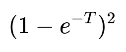
The probability that both components fail before the next inspection (i.e., within time T) is
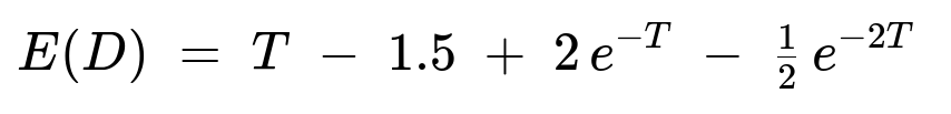
The expected downtime D (the amount of time the system is down between inspections) can be shown, after integration and simplifying, to be
Comprehensive Explanation
Part (a): Probability the system goes down between two inspections
System failure criterion The system is in parallel configuration, so it fails only if both components have failed. Since each component has an exponentially distributed lifetime with rate 1 (density e^(-x) for x ≥ 0), the joint distribution is f(x,y) = e^(-(x+y)) for x,y ≥ 0.
Event of interest We inspect at times 0 and T. A failure occurs between two inspections if both X ≤ T and Y ≤ T. Because X and Y are independent exponentials with parameter 1:
P(X ≤ T) = 1 - e^(-T)
P(Y ≤ T) = 1 - e^(-T)
Hence the probability that both fail by time T is

Memoryless property The exponential distribution’s memoryless property helps confirm that once a failed component is replaced at time T, it is “as good as new” for the next interval.
Part (b): Expected amount of time the system is down
Definition of D Let D denote how long the system is non-functional over the interval [0, T]. If both components fail before time T, the system will be down from the moment of the second failure until we reach time T (the inspection time at which the failed component(s) get replaced).
Mathematically, D = T - max(X,Y) if X ≤ T and Y ≤ T D = 0 otherwise
Setting up the double integral The expectation E(D) is
[
\huge E(D) ;=; \iint_{{0 \le x \le T,,0 \le y \le T}} \bigl(T - \max(x,y)\bigr),e^{-(x+y)},dx,dy. ]
By symmetry and careful partitioning of the integration region (x > y versus y > x), one can write
[
\huge E(D) ;=; 2 \int_{0}^{T} \int_{0}^{x} \bigl[T - x\bigr],e^{-(x+y)},dy,dx. ]
Carrying out the inner integral (\int_{0}^{x} e^{-y},dy) = 1 - e^(-x) and simplifying leads to:
[
\huge E(D) ;=; 2 \int_{0}^{T} \bigl(T - x\bigr),e^{-x},\bigl(1 - e^{-x}\bigr),dx. ]
Performing the integral After expanding and integrating term by term (or by integration by parts), one arrives at the closed-form solution
The key steps involve splitting it into two separate integrals:
(\int_{0}^{T} (T - x),e^{-x},dx),
(\int_{0}^{T} (T - x),e^{-2x},dx),
then combining them with the correct coefficients.
Consistency checks
If T = 0, then E(D) = 0 as expected (there is no “time interval” at all).
For small T, E(D) is close to zero because the probability of both failing that quickly is small.
The expression remains nonnegative for all T > 0, as an expectation must.

Overall, we see that the memoryless property of the exponential distribution allows us to handle replacements neatly at each inspection, and the symmetry of the problem simplifies the double integral.
Potential Follow-Up Questions
What happens if the rate parameter of the exponentials were λ instead of 1?
You would replace each e^(-x) by e^(-λx) throughout. The probability that both fail by time T would become (1 - e^(-λT))^2, and the expected downtime integral would involve e^(-λx) accordingly. The final expressions for P(X ≤ T, Y ≤ T) and E(D) would then be:
Probability: (1 - e^(-λT))^2
Expected downtime: you would see factors of λ in the integrals, and after simplification, you would get a formula involving e^(-λT) and e^(-2λT). The structure is similar but scaled by 1/λ.
How does the memoryless property specifically influence the result?
Exponential lifetimes are memoryless, meaning that if a component has not failed by some time t, the “remaining” lifetime distribution is the same as at the start. This makes the replacement strategy simple to analyze: at each inspection, any failed component is replaced with a new one whose time-to-failure again has the same exponential distribution. Without the memoryless property, the time-to-failure of a component that has not failed yet would depend on how long it has already survived, making the analysis more complicated.
Could we have computed E(D) by conditioning on the event that both fail?
Yes. One approach is:
Let p = P(X ≤ T and Y ≤ T) = (1 - e^(-T))^2.
Conditional on both failing in [0, T], the downtime is T - max(X, Y).
You would then compute E(T - max(X, Y) | X ≤ T, Y ≤ T) and multiply by p. Because X and Y are independent exponentials truncated at T, you would need the conditional distribution of (X, Y) given X ≤ T, Y ≤ T. It is doable, but the double-integral method often ends up simpler or at least more direct for interview-style problems.
If T is very large, does the system effectively become certain to fail in each interval?
When T is large, the probability (1 - e^(-T))^2 is very close to 1, because e^(-T) becomes negligible. Hence, it is almost certain that both components fail before the next inspection. As for the expected downtime, in that large-T regime, E(D) approaches T minus a smaller correction term. Intuitively, if T is very long, the system will almost surely fail and remain failed for a significant portion of the interval once both components have gone down.
How might this change if the system had more than two components?
For n parallel components each with exponential(1) lifetime, the system fails once all n have failed, so P(failure by T) = (1 - e^(-T))^n. The downtime would be T minus the maximum of all n failure times, and you would handle the corresponding multiple-integral or use other order-statistic properties for exponential distributions. The integrals become more involved, but the logic remains similar.
Can you show a quick Python snippet to numerically verify these integrals?
Below is a simple Monte Carlo approach:
import numpy as np
def simulate_downtime(T, n_sim=10_000_00):
# Generate exponentials for X and Y
X = np.random.exponential(scale=1.0, size=n_sim)
Y = np.random.exponential(scale=1.0, size=n_sim)
# System fails if X <= T and Y <= T
# Downtime = T - max(X,Y) if both <= T, else 0
maxXY = np.maximum(X, Y)
downtime = np.where((X <= T) & (Y <= T), T - maxXY, 0.0)
# Probability of failure
prob_fail = np.mean((X <= T) & (Y <= T))
# Expected downtime
e_downtime = np.mean(downtime)
return prob_fail, e_downtime
# Example usage:
T_val = 1.0
p_fail, eD = simulate_downtime(T_val)
print("Empirical Probability of Failure:", p_fail)
print("Empirical Expected Downtime:", eD)
# Compare to closed form:
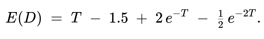
closed_form_p = (1 - np.exp(-T_val))**2
closed_form_eD = T_val - 1.5 + 2*np.exp(-T_val) - 0.5*np.exp(-2*T_val)
print("Closed-form Probability:", closed_form_p)
print("Closed-form E(D):", closed_form_eD)
Such a simulation will typically confirm that for large n_sim, the empirical results match the closed-form answers.
Below are additional follow-up questions
What if the inspection time T itself is random rather than fixed?
In many real-world systems, inspection times might not be strictly fixed intervals. For example, there could be delays or early inspections triggered by external factors. Let’s suppose T is itself a random variable (for instance, uniformly distributed between some bounds or following an exponential distribution with parameter α). The question is then how to compute:
The probability that the system fails before the random inspection time.
The expected downtime in this scenario.
Detailed Answer
When T is random, the events “X ≤ T” and “Y ≤ T” must be integrated over the distribution of T. Let’s call the distribution of T by F_T(t) = P(T ≤ t). The probability the system fails before an inspection is:
P(X ≤ T and Y ≤ T) = ∫[0 to ∞] P(X ≤ t and Y ≤ t) dF_T(t).
Because X and Y are exponential(1), P(X ≤ t and Y ≤ t) = (1 - e^(-t))^2. If T has a PDF g(t), then:
P(failure) = ∫[0 to ∞] (1 - e^(-t))^2 g(t) dt.
A key pitfall is that one must correctly model the distribution of T. If T can be very large with positive probability, then (1 - e^(-t))^2 is near 1 for large t, which can increase the chance of failures significantly.
For the expected downtime, we’d do a similar integral:
E(D) = ∫[0 to ∞] E(D | T = t) g(t) dt,
where E(D | T = t) is what we computed under the assumption T is fixed (T - max(X,Y) if both fail, 0 otherwise). A subtlety arises if T has a distribution that places significant mass on small t-values, because then the probability of failure in a short interval is small, but the distribution might have a “tail” that occasionally results in a large T, increasing both the chance of failure and downtime. Handling these extremes requires carefully ensuring the correct distribution for T is used.
How do we compute the variance of the downtime?
While the expectation of the downtime is crucial, sometimes the variability of downtime is equally important for risk assessment. Thus, one might ask for Var(D), the variance of D, to capture how spread out the downtime is around its mean.
Detailed Answer
Recall D = T - max(X, Y) when both X and Y are less than T, and D = 0 otherwise. To find Var(D), we need E(D^2) - [E(D)]^2.
First, compute E(D^2). This will be an integral similar to E(D), but we have (T - max(x, y))^2 in the integrand: E(D^2) = ∫[0 to T] ∫[0 to T] (T - max(x, y))^2 e^(-(x + y)) dx dy.
We can split it into two regions: x > y and x < y. After adjusting for symmetry, we get a single integral with the relevant expression. We would integrate term by term to obtain a closed form in terms of T, e^(-T), and e^(-2T).
Once E(D^2) is found, Var(D) = E(D^2) - [E(D)]^2. Subtlety arises in ensuring each piece of the integral is correctly accounted for, particularly the boundary conditions x = T or y = T. Another potential pitfall is not remembering that D can be zero if only one or neither component fails before T.
The main real-world significance of variance is that even if the mean downtime is moderate, a large variance means there could be unexpected long periods of downtime. Thus, risk-averse industries often want to minimize not just expected downtime but also its variability.
How would results change if one component is replaced immediately upon failing, but the other is only replaced at inspection?
Sometimes a system has a partial redundancy policy: if one component fails at any point, it is replaced right away, while the other is replaced only at scheduled inspection times. This question significantly changes the distribution of the second component’s failure time (or the system’s failure time, if the second fails too quickly).
Detailed Answer
Component A is replaced upon failure instantly. That means whenever A fails, it is replaced with a brand-new exponential(1) lifetime.
Component B is replaced only at time T if it has failed. Otherwise, it keeps running.
In this scenario, the system fails only if B fails while A is down. But because A is immediately replaced, the system effectively always has at least one “fresh” exponential component after any A-failure event. The question then becomes: what is the probability that B fails at some point, while A is also in a failed state (a very brief instant in many real-world assumptions, but for modeling, we consider minimal repair times or we might consider a small repair time δ)?
A key pitfall is misapplying the original formula that both fail by T. Because A’s lifetime distribution “resets” every time it fails and is replaced, it’s not as straightforward as the plain (1 - e^(-T))^2 calculation.
One could model this via a continuous-time Markov chain approach:
State (0) = both working.
State (1) = B failed, but A working.
State (2) = A failed, but B working.
State (3) = system down (A and B both failed simultaneously).
Then solve for the probability of hitting state (3) before time T. The memoryless property helps define transition rates, but the immediate replacement of A implies a transition from state (2) back to (0) with some rate if the repair time is not exactly zero. If it is truly instantaneous, the system can’t remain in the “A failed alone” state for any positive time, which simplifies to B failing first and A failing at exactly the same instant. The mathematics can become subtle if not approached carefully.
Could correlated lifetimes be modeled instead of independent X and Y?
In reality, the two components might be subject to the same environmental stresses (e.g., temperature surges, voltage spikes). This can introduce correlation in their time-to-failure distributions.
Detailed Answer
If the components’ lifetimes X and Y have a joint distribution that is not simply f(x)f(y), then P(X ≤ T and Y ≤ T) = ∫[0 to T] ∫[0 to T] f_{X,Y}(x, y) dx dy cannot be factorized.
Correlation can either increase or decrease the chance of both failing before T. For example, if the two components are positively correlated (subject to the same shocks), the probability that both fail in a short period is higher than in the independent case.
The expected downtime integral likewise becomes: E(D) = ∫∫ (T - max(x, y)) I(x ≤ T, y ≤ T) f_{X,Y}(x, y) dx dy, but now we must handle the joint density with correlation.
A common pitfall is to keep using (1 - e^(-T))^2 when in fact that formula only holds under independence. For correlated exponentials (e.g., via a copula), the result can differ substantially.
From a real-world standpoint, ignoring correlation can lead to underestimating the probability of simultaneous failures, which can be catastrophic if these parallel components are crucial for safety.
How do we model partial failures or degradation states?
In some systems, a component might not abruptly “fail” but degrade into a partly functioning state. The question is how that affects the definition of “system is down” if we have partial capacity but below some threshold.
Detailed Answer
Instead of a binary working-or-failed model, we introduce states such as “fully functioning,” “degraded,” and “failed.” If each component can degrade, the system might still operate if at least one is fully functioning or even if both are degraded but can combine their partial functionality.
The classic exponential(1) distribution for “time-to-complete-failure” might be replaced with a continuous-time Markov chain or a semi-Markov process that tracks the transitions from working → degraded → failed. Each transition can still have an exponential holding time if memorylessness is assumed.
The probability of system downtime becomes more nuanced: the system is down if the combined states of the two components do not meet the minimal operational threshold. Over a time horizon 0 to T, we must track the chain of states.
A major pitfall is oversimplification by ignoring the possibility that even if a single component is partially degraded, the system might still be considered “up” but less reliable. Realistically, reliability analysis can require a large state space model, each with its own transition rates.
What if the cost of downtime is not simply proportional to the length of time, but escalates with time?
In practice, a system that is down for longer might incur disproportionately higher costs over time (think of lost revenue or potential safety hazards mounting the longer the system is offline). Then we care about E(g(D)) for some cost function g rather than just E(D).
Detailed Answer
Examples of cost functions:
g(D) = c*D (linear cost).
g(D) = c*(D^2) (quadratic penalty for extended downtime).
g(D) = c1 if 0 < D < d, and c2 >> c1 if D ≥ d (a threshold penalty after a certain downtime).
To compute E(g(D)), you would replace (T - max(x, y)) in the integrals with g(T - max(x, y)). The rest of the approach is similar, but the integrals might not have as clean a form.
The pitfall is mixing up E(D) with E(g(D)). Minimizing E(D) is not always the same as minimizing E(g(D)), especially if g is nonlinear. System design might be drastically different depending on whether you care about average length of downtime or the cost function that heavily penalizes extended outages.
Is there a closed-form expression for the distribution of max(X, Y) given that both are exponential(1)?
Sometimes we’re asked not just for the probability or the expectation of downtime, but the entire distribution of downtime. This requires knowledge of the distribution of max(X, Y).
Detailed Answer
For two independent exponential(1) random variables X and Y, the PDF of max(X, Y) is: f_max(z) = 2 e^(-z) - e^(-2z).
This follows from P(max(X, Y) ≤ z) = P(X ≤ z, Y ≤ z) = (1 - e^(-z))^2. Differentiating yields the PDF.
The downtime D = T - max(X, Y) if max(X, Y) ≤ T; otherwise 0. So to find the distribution of D, we note that D is 0 if max(X, Y) > T. Otherwise, it’s T - z for 0 ≤ z ≤ T.
We can write P(D ≤ d) for 0 ≤ d ≤ T as P(D ≤ d) = P(T - max(X, Y) ≤ d) = P(max(X, Y) ≥ T - d). By shifting the variable properly, we can derive the distribution function for D.
A pitfall might be forgetting that D is 0 with some probability. The distribution of D is thus a mixture: there is a point mass at 0 (the probability that max(X, Y) > T) plus a continuous part for 0 < D < T.
This is crucial if you need a complete risk assessment or you want to compute more advanced functionals like quantiles of downtime.
What if there are multiple inspections within the same interval T?
Sometimes an inspection might happen at time T/2 (a mid-interval check) and then again at time T. The question is how that changes the probability of a complete system failure within the overall timeframe [0, T].
Detailed Answer
If partial or additional inspections occur, each inspection can reset the failed components to “as good as new” at those inspection times. This breaks the interval [0, T] into subintervals, say [0, T/2] and [T/2, T].
The probability the system fails in the first subinterval is P(X ≤ T/2 and Y ≤ T/2) = (1 - e^(-(T/2)))^2. If the system does fail in [0, T/2], we might track how long it remains down in that subinterval. But then at T/2, both failed components are replaced, so the second subinterval [T/2, T] starts fresh with two working components again.
The final probability of a system failure at any point in [0, T] could be approached by computing the probability the system fails in the first subinterval or in the second subinterval (independent after replacement). One would have to carefully account for the possibility the system is already down at T/2. If the system fails in [0, T/2], it remains down until T/2, at which point it’s repaired. Then there’s a new chance for failure in [T/2, T].
A pitfall is incorrectly adding probabilities rather than using “probability of at least one failure event in the union of subintervals.” Because of the memoryless nature, the subinterval events can be treated somewhat independently once repairs happen, but the total downtime is the sum of any downtime in the first subinterval plus any downtime in the second. Calculations can get more complex if there are multiple mid-interval inspections.