
ML Interview Q Series: Analyzing Joint Lifetimes with Poisson Distributions: Marginals, Independence, Correlation

Browse all the Probability Interview Questions here.
11E-6. The joint probability mass function of the lifetimes (X) and (Y) of two connected components in a machine can be modeled by

(a) What are the marginal distributions of (X) and (Y)? (b) What is the joint probability mass function of (X) and (Y - X)? Are (X) and (Y - X) independent? (c) What is the correlation between (X) and (Y)?
Short Compact solution
(a) By summing out the other variable, we obtain:
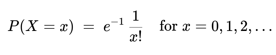
The marginal distribution of (X) is Poisson with parameter 1:
The marginal distribution of (Y) is Poisson with parameter 2:
(b) Defining (V = Y - X) leads to:
The joint pmf of (X) and (Y - X) is

Because this factorizes into (P(X=x)\times P(Y-X=z)), (X) and (Y - X) are independent.
(c) Using (Y = X + (Y - X)) and independence, we have (\mathrm{Var}(X)=1), (\mathrm{Var}(Y)=2), and (\mathrm{Cov}(X,Y)=1). Thus the correlation is

Comprehensive Explanation
Part (a): Marginal Distributions
To find (P(X=x)), we sum the joint pmf (p(x,y)) over all valid (y). From the problem statement, (y) ranges from (x) to infinity for each (x). So,
(P(X=x)) = sum over y from x to infinity of [ e^(-2) 1/(x!) 1/((y-x)!) ].
We can rewrite y-x as k, which runs from 0 to infinity:
Factor out e^(-2)/ x!.
The remaining sum is sum from k=0 to infinity of 1/k!, which equals e.
Hence, P(X=x) = e^(-2)/ x! * e = e^(-1)/ x!.
Since e^(-1)/ x! for x=0,1,... matches the form of a Poisson(1) distribution, it follows that X ~ Poisson(1).
Similarly, to find (P(Y=y)), we sum over x from 0 to y:
(P(Y=y)) = sum over x=0 to y of [ e^(-2) 1/(x!) 1/((y-x)!) ].
Factor out e^(-2)/ y!, and note that sum_{x=0 to y} of [ y!/( x!(y-x)!) ] = 2^y. So:
P(Y=y) = e^(-2)/ y! * 2^y = e^(-2)*2^y / y!.
This is precisely the probability mass function of a Poisson(2). Hence Y ~ Poisson(2).
Part (b): Joint pmf of (X) and (Y-X), and Independence
Define V = Y - X. Then:
p(X=x, V=z) = p(X=x, Y=x+z).
By direct substitution:
p(X=x, Y=x+z) = e^(-2) 1/( x! ) 1/( z! ).
Because x = 0,1,... and z = 0,1,..., we see that
p(X=x, V=z) = e^(-2)/[ x! z! ].
Now, observe:
Summing out x for a fixed z gives P(V=z) = e^(-2)/ z! sum_{x=0 to infinity} (1/x!).
sum_{x=0 to infinity} (1/x!) = e.
So P(V=z) = e^(-2)/ z! * e = e^(-1)/ z!.
That is Poisson(1) for V. We already know X is Poisson(1). Now check if p(X=x, V=z) = P(X=x) P(V=z):
P(X=x) = e^(-1)/( x!).
P(V=z) = e^(-1)/( z!).
Their product is [ e^(-1)/( x!) ] [ e^(-1)/( z!) ] = e^(-2)/ [ x! z! ], which matches p(X=x, V=z).
Hence X and Y - X are independent, each Poisson(1).
Part (c): Correlation Between (X) and (Y)
Recall that correlation(X, Y) = Cov(X, Y) / sqrt(Var(X) Var(Y)).
We have:
E(X)=1, Var(X)=1 (Poisson(1)).
E(Y)=2, Var(Y)=2 (Poisson(2)).
Also Y can be written as X + (Y - X). Since Y-X is independent of X, Cov(X, Y - X) = 0. Then
Cov(X, Y) = Cov(X, X + (Y - X)) = Cov(X, X) + Cov(X, Y - X) = Var(X) + 0 = 1.
Thus
rho(X, Y) = 1 / sqrt(1 * 2) = 1 / sqrt(2).
Potential Follow-Up Questions
Why does the summation approach show that X and Y have Poisson marginals?
When we sum out one variable from the joint pmf, we leverage the factorial expansions. For X, the sum reduces to the series sum_{k=0 to infinity} 1/k!, which is e. For Y, the binomial coefficient summation sum_{x=0 to y} [ y!/(x!(y-x)!) ] equals 2^y. These classic results are the foundation of deriving the Poisson forms.
Could we have recognized a hidden decomposition earlier?
Yes. Notice that p(x, y) depends on x and (y - x), suggesting Y can be seen as a sum of two independent components. Indeed, we identified Y - X as another Poisson(1) random variable, independent of X.
How do we compute the covariance more directly from the definition?
Cov(X,Y) = E(XY) - E(X)E(Y). One way to find E(XY) is to use Y = X + (Y - X). Then XY = X(X + (Y - X)) = X^2 + X(Y - X). Taking expectation:
E(X^2) = Var(X) + [E(X)]^2 = 1 + 1^2 = 2.
E(X(Y - X)) = E(X) E(Y - X) = 1 * 1 = 1 (by independence and the fact that Y - X ~ Poisson(1)). So E(XY) = 2 + 1 = 3, and thus Cov(X,Y) = 3 - (1)(2) = 1, matching the simpler argument above.
What if we tried to simulate data from this distribution in Python?
A direct approach:
Sample X ~ Poisson(1).
Independently sample Z ~ Poisson(1).
Let Y = X + Z.
Then (X, Y) has the desired joint distribution.
import numpy as np

n = 10_000_000  # large sample
X_samples = np.random.poisson(1, n)
Z_samples = np.random.poisson(1, n)
Y_samples = X_samples + Z_samples

# Check means and correlation
print("Mean of X:", X_samples.mean())
print("Mean of Y:", Y_samples.mean())
corr = np.corrcoef(X_samples, Y_samples)[0, 1]
print("Correlation between X and Y:", corr)
This Monte Carlo approach numerically confirms that X has mean ~1, Y has mean ~2, and correlation is close to 1/sqrt(2).
Edge Cases and Practical Significance
Edge Case: X=0 or Y=X. These are accounted for by the pmf structure directly, and the summations start at 0.
In practice, seeing Y as X + (Y - X) with two Poisson(1) terms is the quickest conceptual route to all the properties: marginals, independence, and correlation.
Such a decomposition appears often in Poisson processes (e.g., splitting or combining arrival streams).
Everything consistently confirms that X ~ Poisson(1), Y ~ Poisson(2), X and Y - X are independent (both Poisson(1)), and rho(X, Y) = 1 / sqrt(2).
Below are additional follow-up questions
How would you confirm that the joint pmf is valid (i.e. sums to 1) without relying on known Poisson facts?
Answer:
One way to verify the joint pmf is valid is to show that the total probability sums to 1 when we sum over all valid (x, y). In this particular setup, x can take values 0, 1, 2, …, and for each x, y must be at least x. So you would compute:
Sum over x=0 to infinity of [ Sum over y=x to infinity of p(x, y) ].
Substitute p(x, y) = e^(-2)*1/(x!)*1/((y - x)!). Then let k = y - x, so k = 0, 1, 2, …, and y = x + k:
The inner sum becomes: sum_{k=0 to infinity} [ e^(-2)*1/(x!)*1/(k!) ].
This equals e^(-2)*1/(x!) * sum_{k=0 to infinity} [1/(k!) ].
The series sum_{k=0 to infinity} [1/(k!)] = e.
Hence, for each x, the inner sum is e^(-2)*1/(x!) * e = e^(-1)/ x!. Next, the outer sum over x=0 to infinity of [ e^(-1)/ x! ] also sums to 1 because sum_{x=0 to infinity} [1/x!] = e, and multiplying by e^(-1) yields 1. This confirms normalization without explicitly invoking the fact that X and Y individually follow Poisson distributions. A potential pitfall here is forgetting that y must start from x (not from 0) and inadvertently summing over an incorrect domain. Doing so would alter the sum or lead to contradictions in the indexing.
How could we handle the scenario if data arrives with potential measurement errors (for instance, sometimes Y < X in the recorded data)?
Answer:
In practice, sensor or logging errors might lead to cases where one observes Y < X, which the given pmf deems impossible (probability 0). A few strategies to handle this:
Data Cleaning or Outlier Handling: If these events are rare, you might treat them as outliers and remove them, especially if you trust the theoretical model that Y >= X always.
Model Refinement: If there is a non-negligible fraction of observations with Y < X, you might need to revise the assumption that Y = X + (something). Real machines might have complexities leading to different distributions altogether.
Robust Likelihood Approaches: Sometimes, you might apply a robust likelihood method that downweights or adjusts improbable observations. Alternatively, a measurement error model could be introduced, perhaps with a small probability that the observed data is flipped or misreported.
A subtle real-world issue is that if measurement devices can systematically misread one of the components, ignoring those cases might bias parameter estimates. Practical solutions often require domain knowledge to see if the “impossible” measurements come from sensor drift, miscalibration, or genuine process anomalies.
Suppose you only observe (X, Y) pairs. How would you estimate the parameter(s) in a real-world setting?
Answer:
Since X and Y are each Poisson, with rates 1 and 2 respectively, a straightforward approach is to:
Collect a sample of observed (x_i, y_i), for i=1,...,N.
Estimate the mean of X by x̄ = (1/N) sum_{i=1 to N} x_i.
Estimate the mean of Y by ȳ = (1/N) sum_{i=1 to N} y_i.
Given the theoretical model, one would expect x̄ ~ 1 and ȳ ~ 2. So the maximum likelihood estimates for the Poisson rates would be λ̂_X = x̄ and λ̂_Y = ȳ.
Potential pitfalls:
If the sample size is small, the estimates may have large variance.
If some portion of the data does not actually arise from Poisson processes, the estimates can be systematically biased.
If Y < X ever shows up in the data, you must decide how to handle those improbable points.
What happens to the correlation if the rate of X changes while the total rate (X + (Y-X)) remains 2?
Answer:
Imagine you keep Y as a Poisson with parameter 2, but you consider a different decomposition, say X ~ Poisson(λ) and Y - X ~ Poisson(2 - λ). Then Y still ends up with parameter 2 because Y = X + (Y - X). For the covariance:
Cov(X, Y) = Cov(X, X + (Y - X)) = Var(X) + Cov(X, Y - X). If X and Y - X are independent, Cov(X, Y - X)=0. Hence Cov(X, Y)=Var(X)=λ. So Var(X) = λ, Var(Y) = 2, and the correlation = λ / sqrt( λ * 2 ) = sqrt( λ/2 ).
This means if λ is smaller or larger than 1, the correlation changes. With λ=1, correlation is 1/sqrt(2). If λ=0.5, correlation is sqrt(0.5/2) = 1/sqrt(4) = 1/2. If λ=1.5, correlation is sqrt(1.5/2).
Pitfall: One must confirm that the decomposition you choose (X, Y - X) truly matches the physical process. If the machine physically splits the lifetime into two separate Poisson-type components, that might justify changing λ. Otherwise, forcing a mismatch between the model and real data may yield incorrect conclusions about correlation.
How would you explain the independence of X and Y - X to non-technical stakeholders?
Answer:
You can use an analogy of two streams of discrete “events” that together form the total. Think of Y as the total count of events in a combined process with rate 2. Then X is the count of events in the first sub-process with rate 1, and Y - X is the count of events in the second sub-process, also with rate 1. If these sub-processes are truly independent, the number of events in the first sub-process does not influence how many occur in the second. Therefore, you see that the partitioning of a Poisson(2) process into two Poisson(1) processes yields X and Y - X as independent.
Pitfalls in a real system might be correlated sub-processes (for instance, if an increase in one sub-process directly hinders or amplifies the other). If independence is violated, the model that X ~ Poisson(1) and Y - X ~ Poisson(1) independently might not hold.
What if the underlying process had a different waiting time distribution but you still tried to model with Poissons?
Answer:
In real-world machine lifetimes, the assumption that each component’s lifetime or count is Poisson might be violated (for instance, lifetimes can be closer to Exponential or Weibull). The given approach works specifically under the assumption that events (like “failures” or “arrivals”) follow a Poisson process. If the data is not well-approximated by a Poisson mechanism, parameter estimates, confidence intervals, or predictions might be seriously off.
For example, if the actual lifetimes have a long-tail distribution or seasonality, Poisson would underestimate variance or misrepresent peak event times. A step further would be to check the goodness-of-fit with, say, a chi-square test or the Kolmogorov–Smirnov test adapted for discrete distributions.
Pitfall: Blindly applying a Poisson model just because data are counts can lead to incorrect inferences if the counts do not truly exhibit the memoryless and random arrival properties that define Poisson processes.
Could there be overdispersion in real data, and how would it affect the model?
Answer:
Overdispersion refers to the situation where the variance in the observed data exceeds the mean, which is inconsistent with the Poisson assumption that mean and variance are equal. In a real setting, if your empirical variance for X or for Y is significantly larger than their sample means, that signals overdispersion.
Implications:
The Poisson-based confidence intervals for parameter estimation or hypothesis testing become too narrow if you ignore overdispersion.
The correlation estimate might be misrepresented; you may observe spurious patterns that the simplified Poisson model cannot capture.
A more flexible model might be a negative binomial distribution or a compound Poisson process. If the process is truly overdispersed, the assumption X ~ Poisson(1) and Y ~ Poisson(2) can be under question.
Pitfalls are failing to detect overdispersion and incorrectly concluding that the fitted Poisson model is appropriate. This can lead to misguided predictions or risk estimates.
How does the sum of X and Y - X being Poisson(2) relate to properties of the Poisson process?
Answer:
An essential property of Poisson processes is that if you have two independent Poisson random variables, X ~ Poisson(λ1) and Z ~ Poisson(λ2), their sum X + Z is Poisson(λ1 + λ2). Hence if X has parameter 1 and Y - X has parameter 1, their sum is Poisson(2). This property underpins the distribution for Y.
In a real machine-failure context, it might mean there are two independent “failure drivers” or “stressors,” each contributing to the total failure count. Summing them yields a combined rate.
Pitfall: Overlooking that property might lead one to incorrectly treat the sum of two Poissons as a mixture distribution or a complicated multi-parameter model. The simplicity of Poisson sums is a big advantage in modeling arrival or failure processes.
How could you detect from data that Y is indeed X plus another Poisson random variable, rather than something else?
Answer:
Empirical Check of Means and Variances:
If Y is consistently about double the mean of X and if X and Y each have sample variances close to their sample means, that suggests they might be Poisson with the correct rates.
Factorization Test:
Attempt to partition the data into X and Y - X. If they appear roughly independent (no strong correlation, no pattern in cross-plot), and each has a sample mean = sample variance, that is consistent with Poisson(1).
Likelihood-Based Tests:
Formally, define a log-likelihood under the model X ~ Poisson(λ1), Y - X ~ Poisson(λ2) with Y = X + (Y - X). Fit λ1, λ2, check if maximum-likelihood estimates align with the data.
Model Comparison:
Compare this decomposition-based Poisson model with alternatives (like a bivariate Poisson or negative binomial approach) using something like AIC or BIC.
Pitfall: If you do not check independence or do not confirm that Y - X actually follows a Poisson distribution, you could incorrectly adopt the simpler model.
Under what conditions would the correlation not be 1/sqrt(2)?
Answer:
Correlation is 1/sqrt(2) specifically because Var(X)=1 and Var(Y)=2, and Cov(X, Y)=1. If the rates change, or if X and Y - X are not truly independent, or if they do not have Poisson(1) distributions individually, the correlation can deviate.
For example, if X and Y - X were Poisson distributed but correlated (not independent), Cov(X, Y - X) ≠ 0. Then Cov(X, Y) = Var(X) + Cov(X, Y - X) would differ, altering the correlation. Or if the rate for X is not 1, the variance changes, shifting the correlation.
Pitfall arises if you assume everything is “ideal Poisson” and accept 1/sqrt(2) as a universal correlation. Real systems might not match those assumptions, and the correlation would need empirical verification.