
ML Interview Q Series: Analyzing Mixed Distributions: EV & CDF for Capped Payouts from Uniform Damage.

Browse all the Probability Interview Questions here.
An insurance policy for water damage pays an amount of damage up to $450. The amount of damage is uniformly distributed between $250 and $1250. The amount of damage exceeding $450 is covered by a supplement policy up to $500. Let the random variable Y be the amount of damage paid by the supplement policy. What are the expected value and the probability distribution function of Y?
Short Compact solution
Since the damage X is uniformly distributed on the interval [250, 1250], it has a length of 1000, so its density is 1/1000 over that range. The supplement payment Y is 0 if the damage does not exceed $450, and otherwise it is (X - 450) capped at $500. This leads to these key facts:
Y is 0 with probability 0.20, corresponding to the damage range [250, 450]. Y is 500 with probability 0.30, corresponding to the damage range (950, 1250]. Otherwise, Y takes values between 0 and 500 when damage lies between (450, 950], and it does so in a linearly increasing way with density 1/1000 for 0 < Y < 500.
Hence the expected supplement payment is 275, and the cumulative distribution function of Y can be written as 0 for y < 0, then 0.20 + y/1000 for 0 <= y < 500, then 1 for y >= 500 (noting the 0.30 mass at Y = 500).
Comprehensive Explanation
To derive the result, consider the damage random variable X ~ Uniform(250, 1250). The supplement policy covers any amount of damage above 450, but only up to 500. Therefore, we define the supplement random variable Y by:
Y = 0 for X <= 450, Y = (X - 450) for 450 < X <= 950, Y = 500 for 950 < X <= 1250.
Since X has a uniform distribution on [250, 1250], its probability density is 1/1000 for x in [250, 1250] and zero otherwise. We analyze the distribution of Y in three segments:
For 250 <= X <= 450, the damage does not exceed $450, so the supplement pays 0. The length of this interval is 450 - 250 = 200, hence P(Y = 0) = 200/1000 = 0.20.
For 450 < X <= 950, the supplement payment ranges from 0 up to 500, specifically Y = X - 450. The length of the interval is 500, so Y takes on a continuous range of values from 0 to 500 over a length of 500 in X. Because of the uniform density 1/1000, the portion of the total probability in this range is 500/1000 = 0.50.
For 950 < X <= 1250, the damage above $450 can exceed 500, so the supplement pays exactly 500. The length of this interval is 300, so P(Y = 500) = 300/1000 = 0.30.
Putting this together, the distribution of Y is mixed, having point masses at 0 and 500, and a continuous part between 0 and 500. To be precise, for 0 < y < 500, the cumulative distribution function FY(y) accumulates probability from the mass at Y=0 (which is 0.20) plus the continuous part from Y=0 up to Y=y in that region. Because Y in (0, 500) corresponds linearly to X in (450, 450+y), the probability contribution up to Y = y is y/1000.
Thus for 0 <= y < 500, FY(y) = P(Y <= y) = 0.20 + (y/1000).
At y = 500, there is an additional jump of 0.30, accounting for Y = 500. That gives FY(500) = 0.20 + 0.50 + 0.30 = 1, which is consistent with the total probability.
To find the expected value of Y, we sum over the continuous part and the point mass at 500. Over 450 < X <= 950, Y = X - 450 contributes a continuous component, and for 950 < X <= 1250, Y = 500 is a point mass of probability 0.30.
The continuous portion (for 450 < X <= 950) can be integrated. One convenient way is to convert X to Y by noting that Y = X - 450 in that range, so Y goes from 0 to 500. However, you can also integrate in terms of X directly:
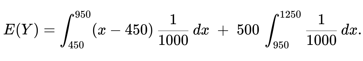
In the first integral, for x in [450, 950], the integrand is (x - 450). In the second integral, for x in (950, 1250], Y is always 500, and the probability mass there is the length 300/1000 = 0.30. Evaluating:
The continuous part is (1/1000) * (1/2)* (950 - 450)2 = (1/1000)* (1/2)* 5002 = (1/1000)* (1/2)* 250000 = 125. The point mass part is 500 * 0.30 = 150.
Adding them gives E(Y) = 125 + 150 = 275.
Potential Follow-up Questions
Explain how to find the variance of Y. One would proceed by splitting Y into its three segments: Y=0 with probability 0.20, Y uniformly distributed between 0 and 500 with probability 0.50, and Y=500 with probability 0.30. You can then compute E(Y2) by integrating over the continuous part and adding the point mass contributions, and use Var(Y) = E(Y2) - [E(Y)]2.
Discuss why Y is called a “mixed” distribution and what that implies in real insurance contexts. The variable Y has both discrete jumps (mass probabilities at 0 and 500) and a continuous region for values in between, meaning it’s neither purely discrete nor purely continuous. In a real insurance situation, any damage below the deductible translates to no payout, and damage that exceeds a certain threshold gets truncated at a policy limit, leading naturally to a combination of discrete probabilities and continuous intervals.
How would these calculations change if the underlying damage distribution were not uniform? You would replace the uniform density by the appropriate density f(x). The probabilities P(Y = 0) and P(Y = 500) would come from integrating f(x) over the intervals where Y remains 0 or hits its maximum of 500. The continuous part would be integrated in the range where the supplement coverage is partial. The same logic applies, but the actual probabilities and integrals would depend on the new density.
Explain how to simulate this scenario in Python. You could generate uniform random samples in Python using numpy.random.uniform(250, 1250, size=N) to simulate damages. Then map each damage value x to y=0 if x<=450, y=x-450 if 450<x<=950, and y=500 if 950<x<=1250. Collect statistics over many samples to empirically estimate the distribution and expected value.
Show a brief code snippet for the simulation:
import numpy as np

N = 10_000_000
X = np.random.uniform(250, 1250, size=N)
Y = np.where(X <= 450, 0, np.where(X <= 950, X - 450, 500))

empirical_mean = np.mean(Y)
empirical_prob_zero = np.mean(Y == 0)
empirical_prob_five_hundred = np.mean(Y == 500)

print("Empirical mean of Y:", empirical_mean)
print("Empirical P(Y=0):", empirical_prob_zero)
print("Empirical P(Y=500):", empirical_prob_five_hundred)
This code verifies the theoretical results for E(Y) and the probabilities at Y=0 and Y=500.
Below are additional follow-up questions
How does the distribution of Y change if the primary policy coverage limit (currently $450) is modified?
One might consider what happens if the primary policy now covers only up to $400 (instead of $450), or perhaps extends coverage to $500. Changing this boundary affects both the probability mass at Y=0 and how large Y can become before it hits the $500 supplement maximum.
If the primary coverage limit decreases from 450 to 400, then the portion of the damage range for which Y=0 shrinks, shifting more probability mass into the region where Y increases continuously from 0 toward the supplement maximum. Specifically, the probability P(Y=0) would then be determined by the length of the interval [250, 400] divided by 1000, which is 150/1000 = 0.15.
At the same time, the continuous portion in which Y = X - 400 spans [400, 900]. That length is 500, so over that region Y ranges from 0 to 500.
Finally, for X > 900, the supplement payment caps at 500.
Hence the overall effect is that P(Y=0) decreases from 0.20 to 0.15, while P(Y=500) remains the same if the total damage range [250, 1250] is unchanged and the supplement limit is still 500. But note that the threshold at which Y hits 500 changes to X=900.
Conversely, if the primary coverage limit were raised above 450, then P(Y=0) would increase, and the probability mass in the middle range would shrink accordingly.
A subtlety is that the uniform distribution range [250, 1250] remains the same; only the policy partitioning changes. Hence it is easy to compute the new probabilities by integrating over the updated intervals. In an interview context, walking through these intervals carefully is key to avoiding mistakes in bounding Y and missing the correct partition thresholds.
What if the total damage can exceed $1250? How would that alter the supplement coverage model?
Suppose real-world scenarios allow for damage potentially greater than $1250, but the data we have only covers up to $1250. In principle, we would need to extend the upper limit of the uniform distribution or switch to a new distribution that accommodates a higher maximum loss.
If we keep the supplement policy capping at $500 beyond the $450 covered by the primary policy, we need to consider that any damage above 950 still leads to Y=500. So if damage can reach beyond 1250, the portion of X>1250 still results in Y=500.
This means the probability mass at Y=500 would be larger, since the interval for which Y=500 now extends beyond 1250.
In real insurance scenarios, water damage might have a “heavy tail,” so the assumption of a strict maximum of $1250 may not be realistic. One must confirm the underlying distribution or find ways to model the tail risk, such as using a Pareto or lognormal distribution for large, infrequent claims.
A pitfall is assuming the same uniform model when in fact damage can be significantly higher than $1250. This might lead to underestimating the probability of extremely large payouts and is a common mistake if one does not validate the domain of the distribution properly.
How would one compute higher moments or the moment generating function of Y?
For more advanced analysis of the supplement coverage, we might need the moment generating function (MGF). Recall that the MGF of a random variable Y is MY(t) = E[e^(tY)].
Because Y is a mixed random variable with point masses at 0 and 500, and a continuous part from 0 to 500, we can write:
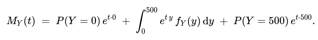
Here P(Y=0) = 0.20, P(Y=500) = 0.30, and fY(y) = 1/1000 over y in (0, 500).
Concretely, the integral from 0 to 500 captures the continuous portion. Since Y maps linearly to X in [450, 950], the density is uniform 1/1000 for that range. We would compute: ∫0500 e^(t y) * (1/1000) dy.
The contribution from Y=0 is simply 0.20 * e^(0) = 0.20.
The contribution from Y=500 is 0.30 * e^(500 t).
Carefully performing this integral for the continuous part yields (1/1000) [ (1/t) ( e^(t y) ) ]0500 if t≠0, plus the point masses. Such computations are commonly required for advanced insurance modeling or pricing more complex derivative-like structures associated with insurance payouts.
A typical pitfall is forgetting to include the point masses or incorrectly calculating the density in the continuous range. Each segment must be accounted for separately.
How can one incorporate an insurance deductible into this model if the policy also required the insured to pay the first $100 of damage?
In many real policies, there is not only a limit on how much the primary coverage pays but also a deductible that the insured must cover before any insurance kicks in. If we insert a $100 deductible, for instance, then:
For damage from $0 to $100 (if such damage is possible), the insured alone pays. That portion does not even go toward the insurance or supplement coverage.
If the damage is between $100 and $450, then the primary policy covers the amount above $100 up to $450 total coverage.
The supplement coverage still begins after $450 is exhausted by the primary coverage, but effectively it may start at X=450 if the insured has already paid the $100.
This can shift probabilities because for X in [250, 100], it may be an impossible range or we might have to re-scale the problem so that coverage only starts after $100 of damage is covered by the insured.
In a uniform distribution scenario that starts at $250, the extra $100 deductible has no effect on the coverage for damage below $250 since we are already starting from $250. But if the uniform distribution truly began at $0 or another lower threshold, the presence of the deductible modifies P(Y=0) and the subsequent calculations of expected coverage.
A subtlety arises if multiple deductibles or multi-layer coverage is involved. Each coverage layer might have its own threshold, which can complicate the analysis. Ensuring that the intervals partitioning X are set correctly is crucial to avoid logical errors in how the distribution of Y is computed.
In practice, how would you validate that the uniform distribution assumption is appropriate for water damage claims?
Real claims data often deviate from idealized distributions like uniform or normal. In practice, you might:
Collect historical claim amounts and perform exploratory data analysis (visualizing histograms, Q–Q plots, or kernel density estimates) to see if a uniform distribution is even remotely plausible.
Fit more sophisticated distributions (e.g., Gamma, Lognormal, Weibull, or Pareto) that are commonly used in insurance for property damage.
Perform goodness-of-fit tests (Kolmogorov–Smirnov, Anderson–Darling, etc.) to assess whether the uniform assumption holds at various levels of significance.
Evaluate the tail behavior explicitly, since water damage claims might cluster around lower amounts but occasionally have large catastrophic claims, making uniform distributions an oversimplification.
A pitfall is to rely on convenience or course materials that mention a uniform distribution without verifying it with real data. In an interview setting, demonstrating awareness of validation techniques and real-world distribution fitting is a strong sign of deeper understanding.
How do correlated risks or repeated damage events impact the distribution of the supplement payouts?
In reality, one property might have multiple water damage events over time, or multiple properties may face simultaneous claims (for instance, if a regional flood occurs). If we assume each damage event is independent and identically distributed, that might not hold in correlated scenarios.
Correlation can increase the frequency and magnitude of claims happening together, particularly if a single catastrophic event affects many homes.
For repeated events at the same property, once a certain claim is filed, subsequent claims in a short timeframe might either be denied or partially covered, depending on policy terms. This leads to more complex models than a single uniform distribution.
From a data modeling viewpoint, you may need a joint distribution or a compound Poisson model where the number of claims is random and each individual claim is drawn from a certain distribution.
A pitfall is ignoring correlation and writing the coverage purely as “uniform(250, 1250).” While it might be acceptable for a simplified single-event scenario, real insurers must consider correlated risk to set premiums and reserves accurately.
How can one extend these ideas to a multi-limit insurance policy, for example, different coverage layers each with its own limit?
In layered insurance (also known as reinsurance structures), you can have multiple layers:
Primary coverage from $0 to $450.
First excess layer from $450 to $950.
Second excess layer from $950 to $1450, and so on.
Each layer covers damage within its specific band, and once that band’s limit is reached, the next layer starts. Y in this problem is essentially the first excess layer from $450 to $950 (capped at $500). If we introduced a second excess layer from $950 to $1450, we would define another random variable, say Z, covering the portion above $950, up to $1450, similarly capping at $500. Each layer can be analyzed the same way, partitioning the distribution of X into intervals.
A major pitfall is mixing up which layer covers which portion of the claim. In an interview, walking through each layer precisely—especially if the question is about the distribution of the total amount paid by all layers—can be tricky. Having a clear picture of the intervals is key:
Layer 1 pays from 0 up to 450.
Layer 2 pays from 450 up to 950 (capped at 500).
Layer 3 pays from 950 up to 1450 (capped at 500). And so on, as needed.
How to generalize the approach if X has a piecewise uniform distribution instead of a single uniform range?
Sometimes real damage data are better represented by a piecewise uniform distribution. For instance, you might have data showing that claims are uniformly distributed from $250 to $600 with one density, but from $600 to $1250 with a different density. Each segment might reflect a different probability of moderate vs. severe damage:
You would split the integration for E(Y) and the calculation of P(Y=0) or P(Y=500) accordingly into multiple intervals matching those density changes.
For each sub-interval, you determine how Y is defined (e.g., still 0 if X <= 450, but X might cross 450 in the first piece or second piece, requiring careful partitioning).
Then you sum up the contributions to probabilities and expectations from each piece.
A subtlety here is ensuring continuity of the total distribution at the transition points. If the piecewise density changes, you must confirm that the total integrates to 1 across the full range. In an interview, be explicit about checking that your piecewise segments add up to the total domain of X, and that each sub-distribution is properly normalized.