
ML Interview Q Series: Analyzing Poisson Thinning and Mixed Poisson Distributions with Uniform Random Rates

Browse all the Probability Interview Questions here.
You sample a random observation of a Poisson-distributed random variable X with expected value 1. The result of this random draw determines how many times you toss a fair coin. What is the probability distribution of the number of heads you will obtain? You then perform a second experiment where you first draw a random number from (0,1), call it U, and then generate an integer from a Poisson distribution whose expected value equals U. Let the random variable X be the integer you obtain. What is the probability mass function of X?
Short Compact Solution
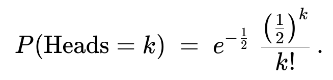
For the first part (where the number of coin tosses is itself a Poisson(1) random draw), the number of heads is Poisson-distributed with expected value 0.5. In other words:
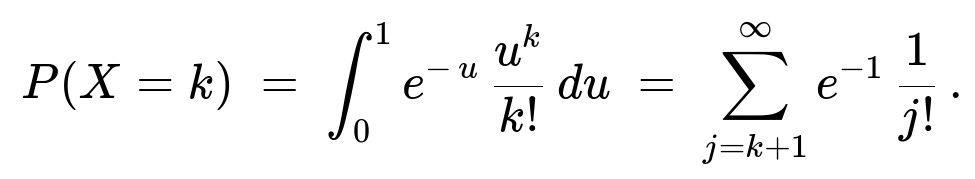
For the second part (where the Poisson parameter is a Uniform(0,1) random variable U), conditioning on U=u gives a Poisson(u) distribution. Deconditioning over u in (0,1) leads to:
Comprehensive Explanation
Part 1: Number of Heads from a Poisson(1)–Determined Coin Toss Count
Let N be a Poisson(1) random variable. We draw a value n from this distribution, and then toss a fair coin n times. We want the distribution of the number of heads, call this random variable H.
By definition, N has probability P(N=n) = e^(-1) * (1^n) / n!, for n=0,1,2,...
Given N=n, we toss a fair coin n times. The count of heads, H, conditional on N=n, follows a Binomial(n, 1/2) distribution, which means: P(H=k | N=n) = (n choose k) * (1/2)^n.
We use the law of total probability to find P(H=k). In text form: P(H=k) = sum over n from k to infinity of [P(H=k | N=n) * P(N=n)].
Substituting the Binomial(n, 1/2) and Poisson(1) PMFs, we get:
P(H=k) = sum over n from k to infinity of [ (n choose k) * (1/2)^n * e^(-1) / n! ] = e^(-1) * (1/2)^k * sum over n from k to infinity of [ (1/2)^(n-k) / (n-k)! ] = e^(-1) * (1/2)^k * e^(1/2) = e^(-1/2) * (1/2)^k / k!.
Hence H is Poisson with parameter 1/2. That is exactly:
The intuitive reason is that a Poisson(1) number of trials, each having a 1/2 chance of success, can be viewed as a thinning of a Poisson process, yielding a Poisson distribution for the successes with mean 1 * 1/2 = 1/2.
Part 2: Poisson with Random Mean U ~ Uniform(0,1)
Now let U be a continuous random variable uniformly distributed on the interval (0,1). We then draw an integer X from a Poisson(U) distribution. So conditionally on U=u, X ~ Poisson(u). We want the unconditional PMF of X.
Conditional distribution: P(X=k | U=u) = e^(-u) * u^k / k! for k=0,1,2,...
Unconditional distribution uses the law of total probability, integrating over all possible values of U in (0,1):
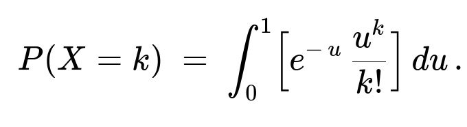
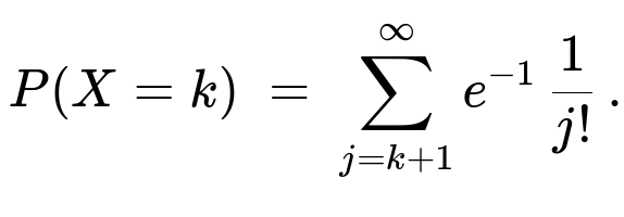
We recognize that the integral ∫[0 to 1] e^(-u) (u^k / k!) du can be interpreted in terms of the incomplete Gamma function or as the probability that an Erlang/Gamma(k+1,1) random variable lies below 1. But from the original snippet, the result can also be expressed more directly as:
To see why this sum form is correct, one approach uses the series expansion or uses integration by parts. Another way is to note:
∫[0 to 1] e^(-u) (u^k / k!) du = [the incomplete gamma expression] = sum_{j=k+1}^∞ e^(-1)*(1/j!).
Hence you get the PMF in that summation form.
Therefore the random variable X can be seen as a “mixed Poisson” distribution: mixing Poisson(λ) over a Uniform(0,1) distribution for λ. And the final expression shows that for each nonnegative integer k, P(X=k) is the tail of the Poisson(1) series starting from j=k+1 onward.
Possible Follow-Up Questions
What is the intuition behind “thinning” in Part 1 and how does it relate to the Poisson(1/2) outcome?
When you have a Poisson process with rate 1 and each event in that process is independently “kept” with probability p=1/2, the resulting process of “kept” events is Poisson with rate p. In the coin-toss setting, the coin tosses (with probability of heads = 1/2) can be viewed as thinning events of the original Poisson(1) process for the total number of trials. The expected number of successes is 1 * 1/2 = 0.5.
Could the result in Part 1 change if the coin is biased?
Yes. If the coin had probability p of landing heads (instead of 1/2), the resulting distribution for the number of heads would be Poisson(λp) when the number of trials follows Poisson(λ). For instance, if N is Poisson(1) and each toss is heads with probability p, then the number of heads would be Poisson(1*p).
Why does mixing a Poisson distribution with a Uniform(0,1) parameter yield the summation form in Part 2?
The mixture distribution arises by integrating the Poisson(λ) PMF against the density of λ. Here, λ = U is uniform(0,1). The integral ∫ e^(-λ)(λ^k/k!) dλ from 0 to 1 can be expressed via the incomplete Gamma function or by summation series expansions. In practice, one can derive the result by recognizing that the integral of λ^k e^(-λ) from 0 to 1 is the difference between the full Gamma(k+1) integral from 0 to ∞ (which is k!) and the incomplete portion from 1 to ∞. This translates into the infinite summation starting from j=k+1.
How would you simulate Part 2 practically?
You would first draw a sample u from Uniform(0,1). Then, given this u, draw a Poisson random variable with mean u. This is done by either:
Summation of Poisson PMF up to cumulative thresholds for a given λ = u,
Using a standard library call if available in your language of choice (for example,
np.random.poisson(u)in Python, given u).
Repeating this procedure many times would generate a sample from the correct mixed distribution.
Are there any edge cases or constraints to consider?
In Part 2, since U is uniform on (0,1), you never sample a Poisson with mean larger than 1, so you expect fewer “large” integer outcomes overall. Indeed, the probability mass for larger k values can be nontrivial but tails off faster than a typical Poisson with fixed λ=1. You also need to be mindful of numerical stability when computing the integral or the tail-sum for large k, though in most libraries, direct Poisson generation given u is straightforward.
How might these concepts appear in machine learning applications?
Mixture distributions (like a Poisson with a random parameter) arise in hierarchical Bayesian models. Thinning concepts appear in count-based processes, such as modeling dropout or random sub-sampling in data streams. Knowing these theoretical underpinnings helps interpret multi-level random processes and hierarchical generative models, which are central to some advanced probability-based machine learning approaches.
Below are additional follow-up questions
What if the Poisson parameter in Part 2 was not Uniform(0,1) but instead had a different distribution (e.g. Beta(α,β))? How would that impact the resulting mixture distribution?
If we replace the Uniform(0,1) distribution of U with some other distribution—say Beta(α,β)—the basic setup remains the same: given U=u, X is Poisson(u). However, the unconditional distribution of X becomes a “mixed Poisson” with the mixing distribution Beta(α,β) on (0,1). In that case, we would compute P(X=k) by integrating the Poisson(u) PMF times the Beta(α,β) PDF over (0,1).
Specifically in text form, we would get: P(X=k) = ∫ from 0 to 1 [ e^(-u) (u^k / k!) f_Beta(α,β)(u ) ] du.
This integral can be more complicated to evaluate analytically than the uniform case, though some closed-form expressions exist for special parameter values. In practical implementations, one may have to use numerical integration. A pitfall arises if you attempt to assume the final distribution is still expressible in a simple closed form—this is not always the case unless α and β take on special forms. In real-world scenarios, you must confirm if the Beta parameters truly represent the prior knowledge about the Poisson mean, because an incorrect prior will skew the mixture distribution.
What if the coin tosses in Part 1 were correlated instead of independent? How would that affect the resulting distribution of heads?
When the Poisson-distributed number of trials is followed by correlated Bernoulli outcomes, the simple thinning property breaks. The derivation in Part 1 crucially relies on the independence of each coin toss. If correlations exist (for instance, if one head increases the likelihood of another head), then the distribution of the total number of heads would no longer be a Poisson(1/2).
In fact, with correlation, one would need the joint distribution of heads given N=n, which would not be Binomial(n, p) if the tosses are not independent. The resulting distribution of H could be overdispersed (variance larger than the mean) or underdispersed, depending on the nature of the correlation. A potential pitfall in real-world data is assuming independence of binary events that are subtly correlated (e.g., outcomes in successive trials might depend on each other). This leads to incorrect inferences about the variance of the final count.
How does the moment-generating function (MGF) or probability generating function (PGF) perspective help in analyzing these Poisson mixtures?
For a Poisson-distributed random variable with parameter λ, the probability generating function (PGF) is G_X(t) = exp(λ(t - 1)). When λ is itself random with distribution F, the overall PGF is the expectation of that expression over λ. For instance, in Part 2, if λ = U ~ Uniform(0,1), we have G_X(t) = E[exp(U(t - 1))].
Since E[e^(cU)] for U uniform(0,1) is (e^c - 1)/(c), we can often identify a closed-form expression for G_X(t) or at least a series representation. MGFs or PGFs can simplify the derivation of mixed distributions or help in identifying bounding behaviors (e.g., tail decay).
A pitfall is forgetting that if the moment-generating function does not exist in closed form, a simpler distributional representation may not be readily available. Also, for larger parameter ranges, numeric approximations might be required. In practice, verifying whether the PGF or MGF exists and is finite is important for theoretical analysis (e.g., if heavy-tailed mixing distributions are involved).
Could any numerical stability issues arise when computing P(X=k) for large k in Part 2?
Yes, numerical instability can be a real concern. If k is large, then evaluating e^(-u)(u^k / k!) directly can be problematic in floating-point arithmetic because u^k and k! can become extremely large or small. When integrating over u in (0,1), you might end up with underflow or overflow if you naïvely compute these powers and factorials.
In real-world implementations, one would typically rely on specialized libraries (e.g., scipy.special.gammaln in Python) to compute log factorials accurately or use series expansions with careful summation. Another practical approach is to simulate from the distribution rather than compute exact PMF values if exact probabilities for large k are not strictly required. The pitfall is underestimating the potential for floating-point error and incorrectly concluding the probability is 0 or ∞ if the software does not handle large exponents or factorials carefully.
In Part 2, how does the distribution compare with a standard Poisson(1) distribution in terms of tail behavior?
When U~Uniform(0,1), the resulting mixture distribution for X is more likely to produce 0 than a Poisson(1) distribution would, because often U < 1. Intuitively, the parameter λ is “on average” 0.5, but it can be any value up to 1. This mixture has a somewhat heavier tail compared to a Poisson with a single mean 0.5 but is lighter than a Poisson(1).
Hence, one pitfall is incorrectly assuming that mixing over (0,1) with a mean of 0.5 would yield the same tail properties as Poisson(0.5). In reality, the mixture approach means there is always a chance that U is close to 1, contributing non-negligible mass to higher outcomes. Therefore, in real applications, ignoring this “occasional large draw of λ” can lead to underestimating the probability of large counts.
What if, in Part 1, the Poisson variable with mean 1 is truncated or censored? Could that affect the final head count distribution?
Truncation or censoring of the Poisson variable N would mean we never observe certain values or only partially observe them (e.g., maximum number of coin tosses is limited to some upper bound m). If N is truncated to the set {0,1,2,…,m}, the law of total probability would still apply but the distribution for N is no longer the standard Poisson(1). We would instead have to normalize for the missing tail. Consequently, H given N would still be binomial with parameter 1/2, but the unconditional distribution P(H=k) would no longer be exactly Poisson(1/2).
This can be a real-world issue if there is a maximum capacity to the number of trials (like a limit on how many times an experiment can feasibly be repeated). A subtle pitfall is inadvertently using the standard Poisson(1/2) assumption without adjusting for the truncated Poisson phenomenon, leading to systematically biased predictions of head counts.
Does the order of generating U first (Part 2) and then sampling X differ from, say, generating X first and then drawing a random U post hoc?
Yes, the order is crucial to the definition of the mixture distribution. In Part 2, the process is: (1) Draw U ~ Uniform(0,1). (2) Condition on U = u, and sample X ~ Poisson(u).
That yields a well-defined “Poisson-Uniform” mixture. If you instead generated X from some distribution and then assigned a random U afterwards, you would not match the mixture distribution described in the problem. A subtle confusion might arise if you interpret the parameter as random but not strictly used as the Poisson mean in a forward generative sense.
Pitfalls arise if you mix up prior and posterior concepts in Bayesian interpretations. You might incorrectly assume you can just draw X from some average distribution and then assign a parameter from a uniform distribution, but that would not reflect the same data-generating process. Always keep track of the direction of conditioning: the parameter is chosen first, then the outcome is generated, which is the hallmark of hierarchical (or mixture) models.
How might these distributions behave under limiting conditions, such as letting the Poisson mean go to zero or to a large value?
When a Poisson mean goes to zero, the Poisson distribution collapses toward zero counts (X=0 with very high probability). For Part 1, if the mean of N was extremely small, the number of heads would almost always be 0. In Part 2, if U had support extending close to zero, that increases the chance that X is 0 or 1. Conversely, if the uniform range extended beyond 1 (say to some large number M), you might frequently see large counts of X.
A pitfall is ignoring these boundary scenarios if your application or domain data occasionally allows near-zero or very large Poisson parameters. For example, if in practice you do not truly restrict to U in (0,1) but have U occasionally near 2 or 3, that changes the mixture distribution dramatically, increasing the probability of large outcomes. This is especially important in modeling real-world phenomena such as traffic counts, demand forecasting, or event arrivals where the rate can vary significantly.