
ML Interview Q Series: As a data scientist in a mortgage lending institution, how would you develop a model that predicts the likelihood of borrowers defaulting on their loans?

📚 Browse the full ML Interview series here.
Comprehensive Explanation
Building a predictive model for default risk in a mortgage bank involves understanding the complexities of credit risk, the nature of mortgage data, and ensuring that the solution adheres to regulatory and practical requirements.
Data Preparation and Feature Engineering
Data often comes from various sources such as credit bureaus, internal transactional systems, and third-party demographic databases. To start, relevant data fields might include borrower income, credit score, employment history, loan-to-value ratio, debt-to-income ratio, property type, collateral value, historical payment behavior, and macroeconomic indicators.
After collecting all relevant data, it is important to handle missing or inconsistent values and encode categorical variables. This step might involve analyzing patterns of missingness—whether the data is missing at random or systematically—which can directly impact the model’s performance. Normalizing or standardizing continuous variables can help certain algorithms converge better, although tree-based models generally do not require it.
Careful feature engineering adds domain-specific insights. For example, payment shock features (how much the monthly payment might increase upon an interest rate reset for adjustable-rate mortgages) can be highly relevant. Lagging or differencing certain time-series features can also highlight changes in behavior over time.
Choosing an Appropriate Model
Many algorithms can be used for modeling default risk, but a common baseline approach is to start with Logistic Regression due to interpretability. More complex ensembles, like Gradient Boosted Trees (XGBoost, LightGBM, or CatBoost), often yield better predictive performance but can be more opaque. It is essential to balance accuracy with explainability, especially for compliance and regulatory requirements.
Logistic Regression Core Formula
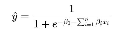
Above, beta_0 is the intercept (also called the bias term) in text form, beta_i are the coefficients (weights) corresponding to each feature x_i, and hat{y} is the predicted probability of default. This predicted probability is typically compared to a threshold—often 0.5, though in practice, a different threshold might be chosen to optimize business metrics or align with regulatory objectives.
With logistic regression, the coefficients beta_i can be interpreted as the log-odds impact of each feature on the probability of default, which is helpful when explaining decisions to stakeholders.
Handling Imbalanced Data
Mortgage default datasets usually have a smaller proportion of defaults compared to non-defaults. This imbalance can lead to a model biased toward predicting the majority class (no default). Potential techniques include oversampling the minority class (default cases), undersampling the majority class, or using synthetic data generation techniques like SMOTE. Class weighting or specialized metrics (such as AUC-ROC, F1-score) can also help address this imbalance.
Model Training and Validation
Splitting data into training, validation, and test sets (or using cross-validation) helps ensure generalization. If there is a time component (i.e., new loans originate over time), performing time-based splits is essential to avoid data leakage. During training, hyperparameter tuning (for instance, using grid search, random search, or Bayesian optimization) can optimize model performance.
Evaluation Metrics
Common metrics include:
Accuracy is often misleading in the presence of class imbalance.
Precision, Recall, and the F1-score are more informative of the trade-offs between false positives and false negatives.
The ROC curve (Receiver Operating Characteristic) and its area under curve (AUC) measure overall ranking performance.
The PR curve (Precision-Recall) is valuable if the minority class is small.
Economic or domain-specific metrics, such as expected profit or loss, also matter. In mortgage lending, you might combine predicted default risk with exposure at default (EAD) and loss given default (LGD) to estimate expected losses and guide loan decisions.
Implementation Example in Python
import pandas as pd
import numpy as np
from sklearn.linear_model import LogisticRegression
from sklearn.model_selection import train_test_split, GridSearchCV
from sklearn.metrics import roc_auc_score, classification_report

# Imagine df is your mortgage dataset with features and a binary target column 'default'
X = df.drop('default', axis=1)
y = df['default']

# Train-test split
X_train, X_test, y_train, y_test = train_test_split(X, y,
                                                    test_size=0.2,
                                                    stratify=y,
                                                    random_state=42)

# Logistic regression with class weights
log_reg = LogisticRegression(class_weight='balanced', max_iter=1000)
param_grid = {'C': [0.01, 0.1, 1, 10]}

grid_search = GridSearchCV(log_reg, param_grid, cv=5, scoring='roc_auc')
grid_search.fit(X_train, y_train)

best_model = grid_search.best_estimator_
y_pred = best_model.predict(X_test)
y_proba = best_model.predict_proba(X_test)[:, 1]

roc_auc = roc_auc_score(y_test, y_proba)
print("Best ROC AUC:", roc_auc)
print(classification_report(y_test, y_pred))
In the above code, class_weight='balanced' is one simple method for tackling class imbalance in logistic regression. You can also explore advanced balancing techniques or ensemble methods for boosting model performance.
Model Interpretability and Regulatory Compliance
For a mortgage default model, it is often critical to ensure transparency. Logistic regression provides a direct understanding of how features affect the odds of default. For more complex models like gradient boosting, techniques such as SHAP (SHapley Additive exPlanations) or LIME (Local Interpretable Model-Agnostic Explanations) can offer insight into feature contributions.
Ensuring compliance requires documenting the model’s development steps, assumptions made, testing for disparate impact (potential biases against protected groups), and regularly monitoring performance drift in production. Auditable logs of model outputs and any overrides or exceptions are often necessary.
How do you handle class imbalance in a loan default scenario?
Class imbalance means default cases could be relatively few. Oversampling default records or undersampling non-default records is one straightforward approach. Alternatively, algorithms like SMOTE can generate new synthetic minority class examples. Another approach is to assign higher misclassification penalties to the minority class. This can be done by adjusting loss functions or using model-specific class weights. Monitoring metrics like F1-score, AUC-ROC, and Precision-Recall curve helps ensure meaningful evaluation in such imbalanced contexts.
Why might you choose a simpler model like Logistic Regression over complex ensembles?
Logistic regression is more transparent and interpretable for regulatory needs. It is easier to explain the effect of each input variable to stakeholders. Even if ensemble methods often yield higher raw predictive accuracy, the lack of interpretability can become problematic when regulators require explicit reasoning behind loan decisions. Additionally, simpler models are less prone to overfitting, especially in smaller datasets, and can be faster to train and update.
How do you ensure the model remains compliant with regulations?
Documenting every step of the modeling process is essential. This includes describing the data sources, the transformations applied, the choice of features, and how they were validated. Maintaining explainability through model-agnostic interpretation methods (like LIME or SHAP) provides transparency. Regular fairness audits on sensitive attributes (race, gender, age, etc.) can uncover disparate impact. Post-deployment, a monitoring pipeline is crucial to track data drift or performance degradation, ensuring the model’s predictions remain accurate and unbiased over time.
What additional considerations are there for production deployment?
Production systems require robust pipelines that handle new data in near-real-time or batch processes. Monitoring is essential so that if data distributions shift or performance degrades, alerts trigger retraining or adjustments. Automated retraining schedules might be employed based on performance criteria. Ensuring data privacy and secure storage (especially for sensitive personal information) is mandatory. Finally, fallback or override policies must be in place to handle unexpected events such as abrupt economic changes or model failures.
Below are additional follow-up questions
How do you incorporate external macroeconomic or temporal factors into the default risk model?
In many mortgage default scenarios, broader economic conditions heavily influence a borrower’s ability to pay. For instance, unemployment rates, interest rates, housing price indices, and GDP growth are all macroeconomic indicators that can correlate with default risk.
To integrate these factors, you might collect historical values of these macroeconomic variables and align them with the loan origination date or payment history date. This process involves joining time-series data with individual loan data on a monthly or quarterly basis. Certain features could include “change in home price index from loan origination date,” “unemployment rate during the quarter of default,” or “change in interest rates over time.”
Potential pitfalls arise if there is a lag between changes in macroeconomic conditions and borrower behaviors. Some borrowers may have saved enough to withstand short-term shocks, while others might default quickly. Time alignment is thus crucial: incorrectly shifting or averaging these indicators can introduce data leakage or inaccurate signals.
With more advanced approaches, you can incorporate dynamic or recurrent neural networks (RNNs, LSTMs) that parse temporal sequences. These models can learn complex dependencies over time, but they require larger datasets and can be harder to interpret. You must also validate these temporal features with an out-of-time test set to confirm the model generalizes well.
How do you account for applicants who were declined a loan and thus have no observed outcome (Reject Inference)?
Reject Inference is a common challenge in credit risk modeling. When you only model outcomes for accepted loans, your dataset lacks the behavior of those who were rejected. This can bias your model, because the model “sees” fewer high-risk cases (assuming the bank’s rejection policy is somewhat successful in identifying risk).
One approach is to infer whether rejected applicants would have defaulted if they had been granted a loan. Methods range from simple assumptions (e.g., assume all rejected are high risk) to more complex statistical techniques:
Augmenting with Bureau Data: Sometimes, external credit bureau records can reveal whether a rejected borrower defaulted elsewhere.
Fuzzy Augmentation: Assign an estimated default probability to rejected applicants using a model built on accepted applicants, then incorporate these pseudo-labels into the main model.
Two-Stage Models: Build a first-stage model to estimate acceptance probability, then a second-stage model for default risk, combining the outcomes.
Potential pitfalls revolve around the correctness of these inferences. Overly simplistic assumptions might skew the model and degrade performance if the reject population differs systematically from the accepted population. Regulatory scrutiny also arises if the model uses unverified assumptions about borrowers who were never actually part of the loan book.
How do you handle partial payments or loan modifications where borrowers do not outright default but restructure?
In practice, not all borrowers that cannot pay in full immediately become delinquent. Mortgage servicers may offer loan modifications, interest rate reductions, or temporary forbearance. Modeling this behavior can be tricky because partial payment or restructured loan data blurs the line between good standing and default.
One method is to define a more granular set of outcomes:
Fully performing
Partial payment
Modified loan
Defaulted
Then, you may choose a multi-class approach or track transitions between states using survival analysis or Markov chain models. For example, in survival analysis, you measure “time to default” as a continuous measure and incorporate the possibility of “censoring” for loans still performing or restructured.
Pitfalls involve data labeling complexity and the need to define when a modification is effectively preventing default versus delaying it. Some loans might re-default after modification, requiring robust historical tracking. Additionally, partial payments might represent different risk levels depending on the ratio of actual payment to scheduled payment, so numerical thresholds need to be carefully tuned.
How can we combine Probability of Default (PD), Loss Given Default (LGD), and Exposure at Default (EAD) to estimate expected losses?
Credit risk management often goes beyond just predicting whether a borrower will default. You also want to quantify the magnitude of the loss in the event of default (LGD) and how much of the principal is outstanding (EAD). The typical relationship is captured by:

Text explanation:
PD is the model’s predicted probability that a given loan will default within a certain time horizon.
EAD is the amount of the loan’s exposure if the loan defaults. For a mortgage, this could be the outstanding balance plus any accrued interest.
LGD represents the percentage of the loan amount that is not recovered in the event of default (for example, if the bank recovers 80% by foreclosure, the LGD is 20%).
All three components can be modeled separately. For instance, one model predicts PD, another estimates the recovery rate or LGD, and a third might forecast EAD based on payment schedules or credit line usage. Integrating these predictions into an expected loss calculation supports capital allocation and risk-based pricing strategies. A major pitfall is ensuring each component is consistently calibrated to the same time horizon and data population.
How do you detect and correct biases that may exist in mortgage default datasets?
Mortgage lending is heavily scrutinized for potential discrimination. Bias can arise if certain protected groups (e.g., by race, gender, age) are systematically underrepresented or if historical lending decisions were influenced by prejudicial factors.
To detect such biases, practitioners can:
Examine distribution of features across different groups to identify skewed patterns.
Assess disparate impact by comparing model outcomes (approval/denial or predicted risk level) across protected classes.
Perform fairness-aware analyses, like measuring demographic parity, equal opportunity, or disparate impact ratio.
To mitigate bias, techniques include:
Pre-processing: Remove or transform sensitive features or use adversarial debiasing methods.
In-processing: Train models with fairness constraints or re-weight examples to level the playing field.
Post-processing: Adjust decision thresholds to achieve fairness metrics without altering the core model.
A subtle pitfall is the risk of “fairness gerrymandering,” where overall fairness might mask pockets of discrimination for certain subgroups. Another issue is inadvertently reintroducing bias if correlated features effectively act as proxies for protected attributes.
What happens if the economic environment or borrower behavior changes drastically after the model is deployed?
Model performance can degrade over time when the underlying data distribution shifts. Sudden macroeconomic shocks (like a recession, a pandemic, or a housing market crisis) can fundamentally alter borrower behavior. This is referred to as “concept drift” or “data drift.”
Common strategies for addressing this include:
Regular Monitoring: Track key metrics such as default rates, average PD, or characteristic distributions. If you detect drift, trigger a deeper investigation.
Adaptive Retraining: Periodically retrain the model on recent data or incorporate online learning methods so the model continuously updates.
Champion-Challenger Framework: Maintain a production model (champion) and test new models (challenger) on incoming data. Promote the challenger to champion if it consistently outperforms.
Pitfalls arise if you do not detect drift quickly enough. You might continue to make suboptimal lending decisions, accumulating risk. Conversely, overfitting to a short-term shock can lead to instability when conditions normalize.
How can calibration techniques help ensure predicted probabilities align with real-world default frequencies?
Even a model that ranks borrowers correctly from most risky to least risky might be poorly “calibrated,” meaning the predicted probabilities do not match actual observed default rates. For instance, a group of borrowers labeled “10% default risk” might end up defaulting 20% of the time in reality, indicating miscalibration.
Techniques like Platt scaling or Isotonic regression can be applied after your classification model is trained to adjust the output probabilities so that they align better with observed frequencies. For example, if you find that your 10% risk bucket historically defaults at 20%, you can correct the model’s output probabilities accordingly.
A key pitfall is failing to maintain calibration over time, especially in dynamic economic conditions. Calibration must be continually monitored. If a crisis suddenly makes default more probable for the same input signals, your previously calibrated model will no longer match the new reality.
What is the difference between building a classification model for default incidence and a regression model that predicts severity of default?
When modeling default risk, it’s common to build a binary classification model (default vs. not default). However, you might also be interested in how severe the default is—perhaps the number of missed payments, the time to cure (if they eventually catch up), or the total amount of loss.
Classification Approach: Provides a probability that default occurs within a specified horizon. This is simpler, focusing on yes/no outcomes.
Regression (or Another Numeric Prediction): Estimates the magnitude of a potential loss or number of payments missed. This might be more complex but can be more informative if you want to plan for expected capital requirements or provisioning.
A pitfall when predicting severity is data labeling: you must define a numeric target that meaningfully measures the severity (e.g., missed payments, principal shortfall, or total losses). Additionally, the model must be carefully validated because the distribution of severity can be skewed—many loans might have minimal losses, while a few have large losses.