
ML Interview Q Series: Assessing Coin Bias: Hypothesis Testing for 550 Heads in 1000 Flips.

Browse all the Probability Interview Questions here.
3. A coin was flipped 1000 times, and 550 times it showed up heads. Do you think the coin is biased? Why or why not?
Explanation and Reasoning in Detail
Why might we suspect a coin could be biased? Intuitively, if we assume a fair coin, we expect the probability of heads pp to be 0.5. Across 1000 flips, the most likely count of heads would be around 500. Observing 550 heads is somewhat higher than 500, raising the question: is this deviation just random fluctuation, or is the coin genuinely biased?
One way to examine whether this result is due to random chance or indicates a real bias is to perform a hypothesis test or to construct confidence intervals. Below is a thorough exploration of these techniques, real-world considerations, potential pitfalls, and related insights.
Hypothesis Testing Perspective
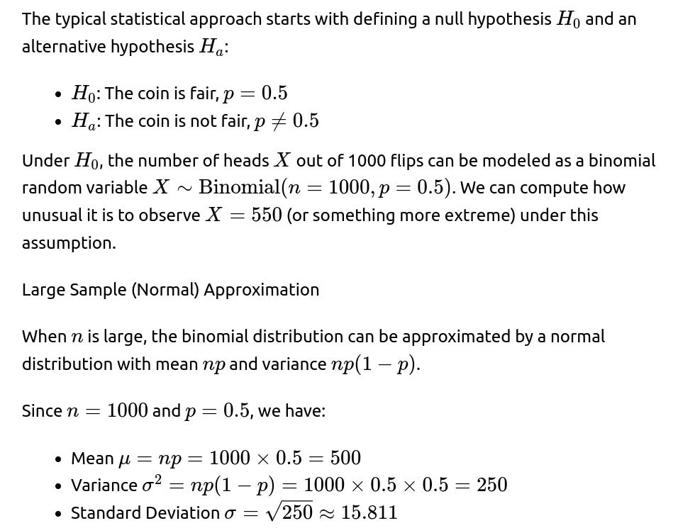

Therefore, by this frequentist hypothesis test criterion, it is likely that 550 heads in 1000 flips is statistically significant evidence to reject the null hypothesis of a fair coin.
Confidence Interval Perspective
Another way to approach the question is via a confidence interval for p. Suppose we estimate p by the sample proportion:

A 95% confidence interval for the true probability of heads can be constructed using the approximate formula:


So the interval is approximately [0.5192, 0.5808]. Notice that 0.5 (the value for a fair coin) is slightly below 0.5192, which suggests 0.5 is not inside the 95% confidence interval. This again indicates that the data provide evidence that the coin may be biased (with heads probability exceeding 0.5).
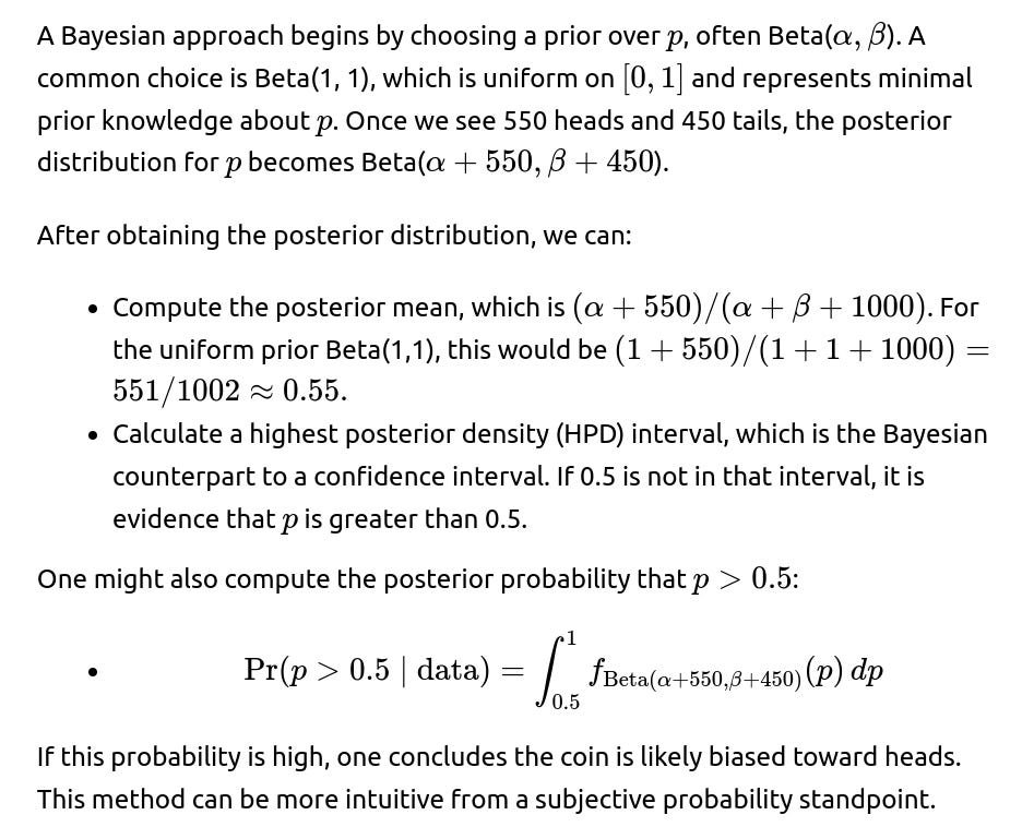
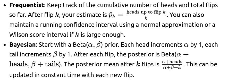
Bayesian Perspective

Regardless of the approach, all these methods converge to the notion that 550 heads out of 1000 is significantly higher than what one might expect from pure chance under a fair coin assumption.
Potential Real-World Pitfalls
Sampling Bias: If the coin flips were not truly independent or if the flipping process was controlled in some manner (e.g., the way a person flips the coin), the results might not reflect the underlying fairness of the physical coin itself.
Multiple Testing or Data Snooping: If we tested many coins and only reported the results of one coin that deviated the most from 50%, that would skew our interpretation.
Practical vs. Statistical Significance: From a purely statistical perspective, 50 out of 1000 extra heads is significant. However, from a practical standpoint, one might ask if that 5% difference has real-world implications. For certain applications, it definitely could (e.g., betting scenarios).
Implementation Example in Python
Below is a quick Python code snippet that uses a standard binomial test in the SciPy library to see whether 550 heads out of 1000 flips is significantly different from 0.5.
import math
from statsmodels.stats.proportion import proportions_ztest

count = 550  # number of heads
nobs = 1000  # number of flips
value = 0.5  # hypothesized proportion

stat, p_value = proportions_ztest(count, nobs, value=value, alternative='two-sided')
print("Z-statistic:", stat)
print("p-value:", p_value)
This will yield a Z-statistic close to 3.16 and a very small p-value, confirming that 550 heads is unlikely to be due to pure chance if p=0.5.
Conclusion of the Main Question
Given the observed number of heads is 550 out of 1000, standard statistical methods (both hypothesis testing and confidence intervals) strongly suggest that the coin is likely biased rather than fair.
How might you use a Bayesian approach to decide if the coin is biased?
Could this result be explained by random chance alone?
Strictly speaking, any one experiment (1000 flips) can still produce 550 heads by chance alone. However, the probability of seeing such a large deviation from the expected value of 500 if p=0.5 is quite small. The exact binomial test or the normal approximation both give very low p-values.
The threshold for deciding “it’s not just chance” typically depends on the chosen significance level. With a standard level of 0.05, we would reject the null hypothesis. With a much stricter threshold (say 0.001), we might still reject the null hypothesis. So while chance alone could produce this result, it is statistically unlikely.
Are there any real-world considerations beyond the raw statistics?
Yes. One important consideration is whether the flips are truly random and independent. If some external factor systematically influences the flips, that might create the appearance of bias in the coin. Also, in practical settings, if this coin is used for critical decisions, even a small deviation from 0.5 could be crucial. In casual settings, one might tolerate or ignore a 55% heads rate because it might be “close enough” to fairness for the purpose at hand.
Another consideration is how stable the estimated probability is if you flip the coin thousands more times. Perhaps 550 out of 1000 was just a lucky streak. Replicating the experiment reduces the chance that an outlier result is guiding our conclusion.
How do we address concerns about multiple comparisons in real data analysis?
If you test many coins or repeat experiments and only highlight the most extreme results, you inflate the Type I error rate. This is known as the multiple comparisons problem. A good practice is to use proper corrections (e.g., Bonferroni, FDR) or pre-register a single experiment so that the interpretation of p-values is statistically sound.
If this single 1000-flip experiment was planned in advance to test one specific coin, then the analysis remains straightforward. But if it was one among many unreported attempts, the significance might be overstated.
Can you show how to do an exact binomial test instead of the normal approximation?
The exact binomial test can be performed in Python with SciPy’s stats.binom_test (in older versions) or newer functions like stats.binomtest. For instance:
from scipy.stats import binomtest

result = binomtest(k=550, n=1000, p=0.5, alternative='two-sided')
print("p-value (exact binomial test):", result.pvalue)
This p-value will generally be quite close to the one from the normal approximation for large n, but it’s considered more accurate since it uses the binomial distribution directly rather than a normal approximation.
Summary of the Statistical Conclusion
With 550 heads out of 1000 flips, the departure from 500 heads is statistically significant. All major statistical approaches (frequentist confidence intervals, hypothesis tests, or Bayesian credible intervals) would point to concluding that p>0.5 at conventional significance levels. Therefore, it is reasonable to state that the coin is likely biased.
Below are additional follow-up questions
Could the coin’s behavior have changed partway through the experiment, and how would you detect that?
A shift in the coin’s “effective bias” during the 1000 flips is a realistic scenario if the physical conditions of flipping changed or if the coin itself got damaged or altered. For instance, maybe for the first 500 flips the coin was fair, and for the last 500 flips it consistently landed heads more often because the flipper’s technique changed (or because the coin got bent slightly).
One way to detect such a change is to perform a change-point analysis. You break the 1000 flips into segments and see if the data in one part of the sequence looks statistically significantly different from the rest. For example, you can:
Split the data at different potential dividing points (say, after 100 flips, 200 flips, and so on). For each split, compute the likelihood of heads vs. tails in both segments and see whether one segment is significantly different from 0.5 or from the other segment.
Use a Bayesian change-point detection algorithm that places a prior on how likely a change could occur and tries to infer both the position and magnitude of the shift in bias. This approach typically uses dynamic programming or Monte Carlo methods (e.g., Markov Chain Monte Carlo).
If a significant shift is detected around a certain flip number, you can hypothesize that the coin’s behavior changed partway through. You might then want to gather more data specifically in the environment or conditions around the suspected shift to verify if the coin itself or the flipping method changed.
A real-world subtlety is that you should confirm that no external factor (like the flipper physically getting tired, flipping from a different angle, or a breeze in the room) caused the shift in outcomes. Distinguishing whether the coin is physically biased from a systematic flipping bias (human behavior) is often challenging.
What if your sample size was much smaller, say 20 flips, but you still observed a higher proportion of heads?
If you only flip the coin 20 times and get 11 heads (55%), you observe the same empirical proportion of heads (0.55) as in the 1000-flip scenario. However, with 20 flips, the total amount of data is far smaller, leading to much higher uncertainty around the true bias. In that case:
A frequentist might do a binomial test and find a p-value that is not small enough to reject the hypothesis of a fair coin. The difference between 11 and 10 heads is typically too small to conclude bias at conventional significance levels because the variance is larger with fewer trials.
A confidence interval for p with just 20 flips would be much wider than for 1000 flips, likely encompassing 0.5 comfortably.
A Bayesian approach (e.g., Beta(1,1) prior updated by 11 heads and 9 tails) yields a posterior Beta(12,10). The credible interval for this distribution is wide, so there would be substantial posterior mass around p=0.5.
Hence, for smaller sample sizes, the random fluctuation is larger relative to the difference between expected vs. observed heads, so you usually cannot confidently conclude the coin is biased. The main pitfall is that with too few flips, the confidence interval or credible interval is wide enough to include a fair coin as a highly plausible scenario.
What if the coin landing on its edge is also a possibility?
Real coins have a tiny (but non-zero) probability of landing on their edge. This possibility slightly complicates the modeling assumptions because standard binomial tests assume all flips result in heads or tails with probabilities that sum to 1. If some fraction of flips land on the edge, the distribution changes:
You might have a three-outcome scenario: heads with probability pp, tails with probability q, and edge with probability 1−p−q. A “fair coin” in a three-outcome sense might still not have p=0.5 and q=0.5 if the edge case is not negligible.
Typically, the proportion of edge outcomes is extremely small (often quoted on the order of 1 in 6000 for certain coin designs and typical flipping methods), so it might be safe to ignore in practical scenarios. But if the coin is thick or the flipping surface is unusual, it might happen more often.

How would you handle suspected correlations between flips?
In a perfect coin-flipping scenario, each flip is an independent Bernoulli trial. However, in reality, there can be correlations—maybe the flipper’s wrist action systematically alternates between strong and weak flips, which might lead to a pattern in the coin’s outcome.
This correlation breaks the standard binomial model, which assumes independent trials. With correlated flips, the variance of the total heads count can be different from the binomial assumption. Some ways to investigate or mitigate correlation effects:
Runs Test: You can check if the sequence of heads (H) and tails (T) shows more (or fewer) runs than expected under independence. A “run” is a consecutive sequence of identical outcomes (like HHH or TT). If the sequence is excessively “clumpy,” it might indicate correlation or changing bias over time.
Block Bootstrapping or Permutation Tests: Instead of assuming each flip is i.i.d., you might do a block bootstrap of the time series to maintain potential short-term correlations, then estimate the distribution of total heads from that resampling.
Model-based Approach: Use something like a hidden Markov model if you suspect the coin’s probability of heads changes in a Markovian fashion from flip to flip. This is more complex, but it might reveal patterns such as a “high-heads” state vs. a “low-heads” state.
The subtlety is that even if the coin is physically fair, the flipping process or environment may introduce correlation or cyclical patterns. Without checking or controlling for correlation, standard binomial-based methods can give misleading p-values and confidence intervals.
Could human biases in reporting the data produce the same effect?
Yes. If a human is recording data manually, there could be systematic errors or biases:
Someone might be more prone to record heads if they look away mid-flip or if they accidentally miss some tails.
In some contexts, the person might subconsciously want the coin to come up heads more frequently, so they might misread borderline cases or quickly glance and assume it’s heads.
To reduce or eliminate such reporting biases, an automated mechanism (like a slow-motion camera or a sensor) can capture the coin’s actual outcome. If manual recording is unavoidable, a double-check or second observer can help ensure data integrity. Auditing the raw data to see if there are suspicious patterns (like no consecutive tails ever recorded, or consistent tallies every 10 flips) can detect anomalies.
How does prior knowledge about coin manufacturing affect your assessment?
If you have prior knowledge that the coin is minted from a reputable source with high manufacturing consistency, you might assign a strong prior belief that p is extremely close to 0.5. In a Bayesian framework, this translates to using a Beta prior heavily concentrated near 0.5.
After observing 550 heads out of 1000 flips, your posterior would still likely shift away from 0.5, but less so than if you had a uniform prior. Whether you decide the coin is “biased” depends on how strong your prior belief was and how persuasive you find 550 heads to be.
Conversely, if the coin is suspect—maybe it’s a novelty coin or you have reason to suspect an unusual weight distribution—you might place a less informative prior or even one that slightly favors p≠0.5. Observing 550 heads would then push your posterior to remain even further from 0.5.
The real-world nuance is that you can combine objective data about coin mass, symmetry, and official minting processes with the flipping data to arrive at a more comprehensive conclusion about bias.
How would you design a more robust experiment to test coin fairness?
Some guidelines for a more robust experiment:
Blinding/Automation: Use a mechanical coin-flipping machine or a high-speed automated flipper that ensures each flip has minimal human involvement. This reduces the possibility that the flipper’s technique biases outcomes.
Randomization of Conditions: If multiple people or settings are involved, randomize which person flips or in which environment flips are done. This keeps external factors from being confounded with the coin’s potential bias.
Large Sample Sizes Over Time: If feasible, gather data from multiple sessions to ensure day-to-day variations in environment don’t systematically favor heads or tails.
Record-Keeping: Use a reliable method for counting heads and tails, such as real-time logging with sensors or multiple observers.
Replications: If you have multiple identical coins from the same mint, you could replicate the experiment across coins and compare results, helping confirm if one coin is an outlier or if all share a bias.
A subtlety here is balancing thoroughness with practicality. Extremely controlled experiments can be expensive or time-consuming, but if the cost of a biased coin is high (e.g., in gambling or critical decision-making), these measures can be worthwhile.
Why might a small p-value still not guarantee the coin is truly biased?
Statistical significance (p-value < 0.05, for instance) does not guarantee that the coin is truly biased. Reasons include:
Type I Error: By definition, even when a coin is fair, there is still a (for example) 5% chance of rejecting the null hypothesis if the significance level is 0.05.
Unrepresentative Sample or Hidden Factors: If the flipping process was not random (e.g., the flips were all done in a way that inadvertently produced more heads), the p-value calculation that assumes independent flips from a fair coin is invalid.
Practical vs. Statistical Significance: Even if the difference is statistically meaningful, in practical terms a coin with p=0.51 or 0.55 might or might not matter depending on context. Statistical significance alone doesn’t measure the real-world impact.
Multiple Testing: If you tested many coins or performed many sequential tests without correction, you might find a “significant” coin by chance.
Understanding that a small p-value points to “strong evidence against the null hypothesis” in that specific test scenario is key. It is not ironclad proof. Additional experiments or confirmations can bolster the conclusion.
What if 550 heads out of 1000 flips was actually part of a marketing claim?
Imagine a scenario where a coin manufacturer claims their commemorative coin is “lucky” because it lands on heads more often. If they present you with an experiment of exactly 1000 flips and show 550 heads, you should question:
Was there any cherry-picking of the data? They might have flipped the coin 20,000 times in total but only reported a subset of 1000 flips that best demonstrated their claim. This artificially inflates the chances of seeing a biased result.
Did they allow independent observers? If the flipping was not monitored by a neutral party, results can be fabricated or selectively recorded.
Was the flipping method truly random? A suspicious technique like “tossing” the coin in a controlled manner can lead to an excess of one face.
If any cherry-picking or non-random flipping is at play, the entire premise of using a binomial test or computing a standard confidence interval breaks down. The potential pitfall is trusting the presented data at face value without verifying the methodology.
How do you handle the scenario where the coin is obviously heavier on one side but the experiments still show near 50% heads?
Sometimes a physically asymmetric coin might still produce close to 50% heads in practice if the flipping process compensates for that asymmetry. For example, if the heavier side might typically face down at landing, but the flipping motion is such that heads or tails remains nearly equally likely.
In such a scenario:
You would still run statistical tests on real-world flipping data to measure actual outcomes. Even if the coin is physically heavier on one side, what matters in practice is whether the flipping process yields 50% heads or not.
If the data from many flips show no significant departure from 50% heads, you can’t reject the hypothesis of fairness based purely on physical asymmetry. The real measure is the flipping outcome, not the coin’s geometry alone.
You might do additional experiments changing the flipping method to see if the coin’s heavier side advantage (or disadvantage) appears under different conditions. If certain flips systematically produce more heads, that suggests the “fairness” depends heavily on how it’s flipped.
This underscores how “biased coin” is context-dependent. A physically off-balance coin might behave as “fair” under some flipping mechanics, while in other flipping styles it might produce a clear bias.
If the coin is indeed biased, how can we estimate the magnitude of the bias?
Once you have concluded the coin is biased, the next question is: “What is the probability of heads, p?” Estimating p typically involves:


If flips are not independent or if there’s a time-varying bias, a single estimate might not capture the whole picture. You’d need a model that allows p to change over time, or you’d sample the coin flipping under known stable conditions.
In practice, if you want to know “how biased” the coin is, you check how far your confidence or credible interval is from 0.5 and whether that difference is practically significant in your use case (e.g., gambling, random selection, etc.).
How would you communicate these results to a non-technical stakeholder who wants a straightforward answer?
When communicating to a non-technical audience:
Summarize the Key Finding: “We flipped the coin 1000 times. We observed 550 heads, which is about 55% heads.”
Explain the Meaning: “Typically, if a coin were perfectly fair, we’d expect 50% heads—about 500 out of 1000. We got 550, which is noticeably higher.”
Convey the Likelihood: “Statistically, the chance that a fair coin would produce at least 550 heads in 1000 flips is quite low—less than 1%.”
Conclusion: “Because the probability is so low, we have good evidence the coin is biased toward heads.”
Caveats: “But there is still a small possibility that this happened by chance alone, or that something in our flipping method influenced the results.”
The subtlety is that “bias” doesn’t necessarily mean extremely far from 0.5. A coin can be slightly biased (e.g., 52% heads) but in large numbers of flips this bias can produce a clear deviation from 0.5 that’s statistically significant.
Could you apply a sequential hypothesis testing framework instead of a single test at the end?
Yes. Instead of flipping the coin 1000 times and then deciding whether it is biased, you could perform sequential hypothesis testing:
Wald’s Sequential Probability Ratio Test (SPRT) is one example. You begin flipping the coin and update your test statistic after each flip. You compare the running statistic to two boundaries: one boundary that favors “the coin is fair” and one boundary that favors “the coin is biased.”
When the running statistic hits one boundary, you make a decision and stop flipping. If neither boundary is met, you keep flipping.
This can be more efficient because if a coin is strongly biased, you might conclude it early with fewer flips, and if it’s very close to fair, you continue collecting data until the evidence is strong enough either way.
A common subtlety is to design your stopping boundaries carefully so you maintain an overall desired Type I and Type II error rate. Another pitfall is that frequent early stopping to declare bias can lead to a higher false-positive rate if the boundaries are not properly calibrated.
Would it matter if the question is about it being biased toward heads vs. a general deviation from 0.5?
Yes. If the only question is “Is the coin biased in favor of heads (i.e., p>0.5)?” that is a one-tailed test. If you are asking “Is the coin not fair (either more heads or more tails)?” that is a two-tailed test:
In a one-tailed test (for p>0.5), the p-value focuses on how extreme the data is in the direction of more heads. You would ignore the possibility of fewer heads as part of the same test. This can yield a smaller p-value if indeed there are many heads.
In a two-tailed test, you include both directions of extremity (much larger than 500 heads or much smaller than 500 heads). This generally doubles the one-tailed p-value if all other assumptions are the same.
A subtlety is that if you had a strong prior reason to suspect bias toward heads only, you might justify a one-tailed test. But many standard procedures default to two-tailed tests unless there’s a compelling rationale for ignoring the other direction. Choosing incorrectly can inflate or deflate the significance of your result.
How does the Law of Large Numbers factor into interpreting 550 heads out of 1000?
The Law of Large Numbers (LLN) states that as the number of independent flips grows large, the sample average (heads proportion) converges to the true probability p. By the time you have 1000 flips, you are in a moderately large sample regime.
If p was truly 0.5, by LLN we’d expect the proportion of heads to be close to 0.5—though “close” is still subject to the usual random fluctuation.
Observing 0.55 suggests the true p may be 0.55 or near that, given the LLN says the average is unlikely to deviate much from the true probability with so many flips.
A subtlety is that “large enough” is relative to how small the difference from 0.5 is and how much variance you can tolerate. Even 1000 flips can exhibit random fluctuations. So the LLN is not a guarantee that you will see exactly 50% or 55%, only that as flips go to infinity, the sample proportion converges to the true p. Observing 550 out of 1000 is consistent with a true p near 0.55, and (as we analyzed) is far enough from 0.5 to raise suspicion about fairness.
How would you approach designing a predictive model that takes coin flips as input features?
If you wanted to build a machine learning model to predict the next flip outcome:
You’d probably start by assuming each flip is i.i.d. with some probability p. The best you could do is predict “heads” with probability p each time. But this is not very interesting—there’s no complex feature set, just repeated flips.
If you suspect non-independence, you might incorporate features like the last few outcomes (Markov property). A model might find patterns that the next flip is more likely to be heads if the last two flips were tails, for example—though physically that’s often just gambler’s fallacy unless the flipping process truly changes.
You could track time-varying patterns. For instance, maybe flips near the end of the day produce more heads for some reason. You’d feed in the flip index or time-of-flip as a feature, and the model might learn a drifting bias.
A subtlety is that you risk overfitting. If you only have 1000 flips, you need to be careful not to chase random noise. Often, a simple approach (estimating a single p or at most a low-order Markov chain) is more robust than a complex neural network for just coin outcomes.
How would you handle the situation where 550 heads are observed, but you believe it might be due to a “hot hand” phenomenon by the flipper?
A “hot hand” phenomenon refers to the idea that success breeds more success—like in basketball, someone who just made a few shots is more likely to make the next shot. Translated to flipping coins, it could mean that if the flipper is on a “hot streak,” they might flip in a way that produces more heads.
While physically questionable in typical coin toss scenarios, if you do suspect a “hot hand” effect:
You’d test for autocorrelation in the sequence. If heads is more likely after a sequence of heads, that suggests a time-varying or state-dependent process.
You might fit a hidden Markov model or some dynamic model that lumps flips into states (e.g., “hot hand state” that yields a higher p for heads and a “cold hand state” with p closer to 0.5).
Even if you do detect a correlation, you’d want to confirm if it’s truly a physical or psychological effect as opposed to random clustering. Clustering can appear by chance.
A subtlety is that a real “hot hand” phenomenon can be extremely difficult to confirm unless you gather a very large dataset showing consistent transitions from cold to hot states. With only 1000 flips, random runs can easily masquerade as hot streaks.
If an online casino used this coin for a 50-50 bet, how should they decide if it’s acceptable?
For an online casino that wants truly fair 50-50 bets, the risk of a 55% heads coin is significant because:
Over a large number of bets, a consistent 5% tilt toward heads can be exploited by savvy players, costing the casino money (if heads is a winning outcome) or angering players (if tails is systematically favored).
The casino might demand that the coin’s bias be estimated precisely (within a tight confidence or credible interval around 0.5). If the interval doesn’t comfortably include 0.5, they might replace or recalibrate the coin (or use a random number generator).
Even small biases matter in gambling contexts. For instance, if large sums are wagered, a 1% or 2% deviation can accumulate large gains or losses.
A subtlety is that casinos typically do not rely on physical coins for large-scale online betting. They often rely on cryptographic random number generators. But if a physical coin is used in a promotional context, the marketing, fairness auditing, and security teams would all want to ensure the coin is effectively 50-50.
What if the “bias” is beneficial in some contexts—would you still care?
Sometimes, a coin with a known slight bias might be beneficial:
Game Mechanics: If you’re designing a board game or a promotional event where you want the coin to have a 55% chance of heads to ensure some outcome occurs slightly more often, you might intentionally design or choose a biased coin.
Research Setting: A slightly biased coin might help measure how people perceive randomness. If you let them guess the outcome of each flip, you can see if they notice the bias.
Performance Tricks: Stage magicians or performers might prefer a coin that reliably turns up heads for a trick.
Even in these scenarios, you need consistent, well-understood performance. The subtlety is that you must keep a record of how the coin was tested and validated so you can rely on the fact it consistently yields the desired 55% heads. If that “55%” starts drifting, your game or performance might not behave as intended.
Could the anomalous result be a simple error like incorrectly counting 50 extra heads?
Data quality mistakes can happen. If someone transcribed or tallied the coin flips incorrectly, that might lead to concluding “550 heads” when the true count was 500. Subtle mistakes that slip into data collection often yield big differences in the final analysis:
Check the raw data (the individual sequence of outcomes) against the summarized count to ensure no transcription errors.
Have multiple counters or a programmatic script double-check the final tally.
Look for suspicious patterns (e.g., if the data show improbable runs or if the ratio of heads to tails changes drastically across short intervals in a manner that conflicts with the reported final total).
A real-world subtlety is that big mistakes can masquerade as important findings. Especially in an interview or an exam scenario, it’s wise to mention verifying data accuracy before delving into sophisticated statistical inferences.
How might you apply a power analysis before flipping the coin?
A power analysis helps determine how many flips you need to detect a given difference from 0.5 with high probability. For instance, if you want an 80% chance (power = 0.8) of detecting a coin that is truly p=0.55 at a significance level of 0.05 in a two-tailed test:
The difference from 0.5 is 0.05. You can use standard formulas or statistical software to estimate how large n must be to reliably detect that difference with a given power.
A subtlety is that if you suspect the coin might be only slightly biased, say 51% heads, you would need a larger n to detect that difference with high confidence. Power analysis ensures you do not waste resources on a too-small sample that fails to detect meaningful biases.
Does the method of flipping (e.g., spinning on a table vs. tossing in the air) affect bias?
Absolutely. The physical method can have a large impact:
Tossing: A standard toss in the air can be fairly random, though technique can matter. Studies have suggested coins can be biased toward the side that starts facing up if the rotation axis is not symmetrical.
Spinning: Coins spun on a table have been shown in some experiments to favor one side due to the dynamics of how the coin interacts with the table surface.
Flicking: Some stage performers can flick a coin in a manner that strongly biases the outcome.
In short, the “true probability” p is not just a property of the coin but of the coin-plus-flip-system. You could find that a physically fair coin has p=0.55 for heads with a certain flipping method and p=0.5 with another. If you truly want to measure the coin’s inherent bias, you need a standardized flipping mechanism that doesn’t systematically favor one face.
A subtlety arises when the interviewer asks “Is the coin biased?” but the real question might be “Is the coin plus flipping method biased?” Distinguishing these is essential if you plan to use the coin in different contexts.
If you discovered a slight bias, how do you correct for it to make decisions fair?
If you want to generate a fair outcome from a slightly biased coin, you can use von Neumann’s procedure:
Flip the coin twice:
If the result is HT, call the outcome “Heads” (in the fair sense).
If the result is TH, call the outcome “Tails.”
If the result is HH or TT, discard and flip twice again.
This procedure, in theory, yields a fair result regardless of the underlying p≠0.5, as long as flips are independent. However, it may waste many flips if p is far from 0.5, because you’ll see HH or TT frequently.

A subtlety is that real-world constraints (time, cost, practicality) might make repeated flipping undesirable. If you need many fair outcomes, discarding half the flips might be too expensive. But from a purely theoretical standpoint, this is a foolproof method to correct for a known (or unknown) coin bias in a random process.
Could “burn-in” flips help remove initial anomalies?
Some experimenters do “burn-in” flips—ignore the first few flips—assuming that once the flipper gets into a consistent flipping rhythm, the bias might stabilize. For example, someone might decide to discard the first 50 flips and only record the subsequent 1000 flips.
The rationale is that early flips might be performed with a different technique (the flipper is warming up or adjusting their motion). If the flipping motion changes systematically, ignoring the early part might yield a more stable measure of pp.
However, there are pitfalls:
You might be discarding genuine data. If the coin is truly biased from the start, ignoring early flips can skew your sample.
If the flipping motion continues to drift over time, ignoring early flips doesn’t solve the deeper problem that the process is not stationary.
A real-world subtlety is that burn-in can help reduce the impact of transients if the flipping method is indeed stabilizing. But it’s no guarantee of fairness if an ongoing trend or correlation is present throughout the flipping sequence.
Is it possible that the extra 50 heads is due to an unusual run in the last few flips?
Yes, it’s possible that the first 900 flips were near 50-50, and the last 100 flips had a streak of heads, pushing the total to 550. This doesn’t automatically mean the coin is biased; it might just be chance. But you’d analyze the distribution of heads across the sequence:
Examine how many heads occurred in the first 500 flips, the second 500 flips, or every 100-flip block.
If the last 100 flips had an abnormally high proportion of heads, you could see if that pattern is improbable compared to typical fluctuations.
Even if the coin is fair, “lucky streaks” can occur. The probability is not zero.
A subtlety is that if you specifically search for streaks only after seeing the results, you’re engaging in post-hoc analysis, which can inflate the chance of concluding there is something unusual. You’d need a proper multiple-hypothesis correction or pre-registered plan specifying “We will examine whether the final 100 flips show a deviation from 0.5.”
How might you incorporate domain expertise about coin flips into the interpretation?
Domain expertise might include:
Knowledge from physics that a coin that starts heads up in your hand is slightly more likely to land heads if you don’t flip it many times in the air.
Empirical research showing typical biases for standard U.S. coins or other currencies. Some studies have found that certain coins systematically come up the same face they started with slightly over 50% of the time.
When analyzing 550 heads out of 1000 flips, domain expertise can refine your prior distribution if you’re using Bayesian methods, or it can shape your experimental design to avoid known pitfalls (e.g., always flipping from the same side up). A subtlety is that the actual observed data might differ from the physics-based expectation if real-world flipping is inconsistent. Observers might not precisely replicate the flipping technique used in controlled experiments.
What if the difference was 550 vs. 500, but the total flips were 10,000?
In that scenario, you have:
10,000 total flips.
550 more heads than expected for a fair coin, meaning you observed 5,550 heads vs. an expectation of 5,000 for a fair coin (p=0.5).


Thus, with more flips, even the same proportion of heads (55%) provides stronger evidence against fairness because your measurement is more precise. A subtlety is that systematic bias or correlation over 10,000 flips might also be more likely if the flipping process has any consistent tilt. But purely from a standard binomial perspective, a 55% outcome in 10,000 flips is a very strong indication the coin is not fair.
In practical machine learning or data science contexts, why do we rarely do coin-toss style tests?
In real data science workflows, we often deal with more complex data (images, text, user behavior logs) and more complex models (neural networks, ensemble methods). We don’t typically rely on “coin flips” unless we’re specifically analyzing a simpler random process. But the fundamental logic behind hypothesis testing for a coin toss is still instructive:
Understanding p-values, confidence intervals, significance levels, and type I/II errors is crucial for interpreting model evaluation metrics.
Many real-world tasks can be reframed in terms of Bernoulli trials (e.g., a user clicking an ad or not). Then we do AB testing or proportion tests analogous to coin flips.
We rely on statistical significance tests to compare conversion rates, engagement metrics, or classification success rates across experiments.
A subtlety is that real-world data seldom obey the i.i.d. assumption perfectly, so we must adapt the tests or modeling approach accordingly. The coin-flip scenario is a simple microcosm that helps illustrate key statistical principles relevant to broader data science tasks.
Could quantum coins or exotic physics lead to unusual distributions?
This might sound far-fetched, but occasionally interviewers pose hypothetical “what if…” questions. A “quantum coin” or a “non-classical coin” could mean some system that does not follow classical probability assumptions:
If each flip outcome depends on a quantum state that can be entangled with some environment variable, you might see distributions that violate the classical model.
In practice, standard minted coins do not exhibit noticeable quantum phenomena at macroscopic scales. So this is more of a theoretical curiosity than a real practical concern.
A subtlety is that in advanced cryptographic or quantum-based random number generation, we rely on sub-atomic processes. But the final aggregated measurement typically still yields outputs that can be analyzed with classical probability. So while the underlying mechanism is quantum, at the macroscale it typically still looks like an i.i.d. Bernoulli process if properly implemented.
How might you handle a coin that is double-headed (or double-tailed) from the start?
A coin with two heads (or two tails) is obviously biased at p=1 (or p=0). If the coin is disguised, you might not realize it at first. In an experiment:
With 1000 flips, you might get 1000 heads. That is conclusive evidence for extreme bias.
But what if the coin occasionally shows tails due to a misinterpretation or a chipping that resembles tails? Or if it’s possible that in certain flipping positions it displays the “underside” of the same face? The outcome might be near 100% but not exactly.
Typically, if we suspect a trick coin, we visually inspect the coin. Relying on flipping data alone is strong but verifying physically can be definitive.
A subtlety is that you might have a coin with a single “two-headed side” but slightly different designs that are not obvious at a glance. Observers might not detect the difference until they carefully look at the coin. Good experimental practice is to physically inspect the coin if extremely unusual results (like 1000 heads in a row) appear.
Could large deviations from 50% be explained by a loaded coin but still be consistent with a normal approximation?

A subtlety is that for p near 0 or 1, the normal approximation gets less accurate because the distribution is skewed. But for moderate biases (like 0.7) and a large n, the normal approximation is still workable, though an exact binomial test or a Beta posterior might be more precise. It clearly indicates a deviation from 0.5 if p=0.7.
If you only recorded the outcome as “is it heads at least 55% of the time or not?” how does that lose information?
Dichotomizing the result—labeling the coin as “more than 55% heads” or “not” instead of keeping the exact count—reduces the resolution of your data. Instead of analyzing exactly how many heads out of 1000, you transform it into a yes/no about whether the proportion exceeded 0.55. This “coarse” approach:
Loses detail about how far above (or below) 0.55 the coin’s heads rate is. Maybe you observed exactly 550 heads or 600 heads or 700 heads; if all those scenarios get labeled “Yes, above 55%,” you cannot differentiate their statistical significance or effect size.
Increases the possibility of borderline misclassification (like 550 heads is just at 55%, so are you labeling that as “yes” or “no”?). A tiny difference in counting could swing that label.
A subtlety is that in some real-world decisions, you only care if the coin’s proportion is above a certain threshold. But from a statistical perspective, you typically lose power by collapsing continuous or near-continuous data into categorical labels.
Why might test quality matter if we want to detect smaller biases?
If the coin is biased at p=0.51 (51% heads), that is a small effect. Detecting such a small deviation from 0.5 at a high confidence level requires:
A large number of flips (sample size). Even 1000 flips might not yield a definitive conclusion for such a marginal difference because the standard deviation around 500 heads is about 15.8. Observing 510 heads might not be a big enough deviation to reject fairness with high confidence.
Careful control of external factors that might introduce additional variance. Even small correlations or mistakes in counting can overshadow a 1% bias.
Possibly a specialized test with higher power or a repeated experiment. A single run of 1000 flips might not suffice; you might do multiple sets of 1000 flips, or go for 10,000 flips in one run.
A subtlety is that real-world constraints might limit how many flips you can do or how carefully you can control conditions. In practice, many biases remain undetected if they are small and overshadowed by random noise or measurement errors.
How would you incorporate a cost-benefit analysis into deciding if 550 out of 1000 flips is “close enough” to fair?
In a cost-benefit analysis, you weigh the cost of continuing with a potentially biased coin against the risk or cost that the bias imposes. For example:
If you’re using the coin for a small-stakes office game, the difference between 50% and 55% heads might not matter. The cost to get a new coin or run more tests might outweigh the slight unfairness.
If the coin is used in a high-stakes gambling context, even a 2% bias might cost or gain tens of thousands of dollars. In that scenario, the cost of doing more flips or procuring a perfectly fair coin is justified.
A subtlety is that organizations often set thresholds for what is “acceptable bias.” For instance, a gaming commission might say “any coin used in official gambling must have a 95% confidence interval that falls entirely within [0.49, 0.51].” If your test indicates an estimated bias of 0.55, that fails the standard, and you would not be allowed to use that coin.
How would repeated flipping over multiple days validate or refute the conclusion?
If you suspect that your first set of 1000 flips was either a fluke or influenced by day-specific conditions (lighting, temperature, flipper fatigue), you might replicate:
Flip the same coin another 1000 times on a different day, possibly with a different flipper or different location.
Compare results. If again you get around 550 heads, that further supports a consistent bias.
If you observe about 500 heads the second time, that might suggest either the first experiment was a statistical outlier or conditions changed.
A subtlety is that day-to-day variations can mask the coin’s true bias or reveal that the coin’s effective bias depends on conditions. If you consistently replicate the 55% figure across multiple well-controlled days, your confidence in the bias conclusion grows significantly.
Could random seeds in simulation approaches mislead the analysis?
If you’re simulating flips or using Monte Carlo methods to approximate p-values or confidence intervals, the choice of random seed can affect the exact numeric results of the simulation. But for large enough simulation runs, the effect of different seeds should be negligible, since the law of large numbers ensures the distribution estimate converges:
Always run enough simulation iterations (e.g., tens or hundreds of thousands) so that the estimated p-value stabilizes and does not vary wildly with different seeds.
If you suspect a bug in the simulation code, try multiple seeds or cross-check the simulation results with exact binomial calculations or an alternative method.
A subtlety is that if the simulation code is flawed (e.g., it incorrectly generates biased random numbers) or if you pick too few iterations, you can get misleading results that either over- or understate significance. Proper code validation is essential.
How might outlier detection techniques reveal something unexpected in the distribution of flips?
Outlier detection typically focuses on identifying data points that deviate significantly from the bulk of the data. In the context of coin flips, the main data is binary—heads or tails. Outliers might not be meaningful in the typical sense. However, if you tracked additional metadata (like how high the coin was flipped, the flipper’s technique rating, or the time between flips), you might notice certain flips were performed abnormally and systematically produced heads or tails:
For example, if you see that the flipper performed “lazy” flips that spun the coin fewer times, you could label these as potential outliers in the distribution of flipping style. Then you check whether those outliers correlated with the coin landing heads more often.
Similarly, if the environment changed drastically (like flipping outdoors in a gusty wind for 100 flips), those flips might be outliers in the sense of environmental conditions.
The subtlety is that “outlier detection” in a standard numeric feature space doesn’t directly apply to heads/tails, but it can be relevant if you track additional continuous variables describing each flip or the environment.
If you wanted an online real-time estimate of the coin’s bias as flips come in, how would you implement that?
An online algorithm updates the estimate of p after each flip without storing all the past data:
A subtlety is that real-time estimates can fluctuate with streaks. If the coin is truly p=0.5, but you see a short run of heads, the estimate or posterior might temporarily shift upward. Only after many flips converge will you see a stable estimate near the true p. If p changes over time (the coin physically warps), your algorithm might lag behind until enough new flips reflect the new bias.
Could the “bias” be beneficial if you needed more heads for a data augmentation technique?
In certain machine learning or data-driven applications, you might want to generate more frequent “heads-like” outcomes if you’re labeling heads as a “positive” class. For example, if you had a simulator that needed more positive examples, a biased coin might ironically help you sample that scenario more often.
However, if your goal is unbiased real-world sampling, you wouldn’t want the coin to produce artificially inflated positives. The subtlety is that in some simulation or augmentation contexts, you might deliberately want a coin (or random generator) that oversamples positives to speed up model training (akin to a biased sampling approach). That is not truly “fair,” but it might be beneficial for the application if you adjust your analysis or weighting accordingly.
Is a 5% difference in heads always “statistically significant” for large sample sizes?

However, the real question is whether that difference is practically significant. If a 0.5% difference has no real impact, you might ignore it. A subtlety is that if you see a tiny difference but with extremely large n, you might reject the null hypothesis in a purely statistical sense yet conclude that the effect size is negligible in practical terms.
Why is it crucial to specify the significance level before seeing the coin flip results?

A subtlety is that in practical machine learning or data science contexts, repeated experimentation can lead to unintentional p-hacking. People keep adjusting parameters or collecting more flips until they get a “significant” result. Proper experimental design demands a pre-specified number of flips (or a sequential testing plan) and a pre-specified significance criterion to maintain integrity.
Could you use confidence intervals alone rather than a hypothesis test?
Yes, many statisticians prefer the clarity of confidence intervals (or Bayesian credible intervals) over simple “reject/not reject” tests. A 95% confidence interval for p that does not include 0.5 implies a p-value below 0.05 for a two-sided test of p=0.5.
Confidence intervals also directly show the plausible range of p. For the coin observed as 550 heads in 1000 flips, you might get an interval like [0.52, 0.58]. You can see that 0.5 is below the lower bound, indicating that a fair coin is not consistent with the data at the 5% significance level.
A subtlety is that intervals can be more intuitive. They communicate both the magnitude of the observed effect (0.55 vs. 0.5) and the uncertainty around that estimate. A single p-value only tells you how surprising the data is under the null hypothesis, not how big or small the effect is.
How do you handle partial flips that are inconclusive?
Occasionally, a flip might land on the floor or get caught in someone’s hand such that the result is uncertain. Some experimenters might choose to re-flip in that scenario, effectively discarding that partial result. Others might mark it as missing data. In any structured experiment:
Decide in advance how to handle ambiguous outcomes (redo or exclude).
If you have too many ambiguous outcomes, you might worry about systematic bias. For example, maybe ambiguous flips were more likely to occur when the coin would have landed tails. That would cause a hidden selection bias.
A subtlety is that ignoring ambiguous flips can bias the sample if ambiguous flips are not random. The safest approach is to define a consistent rule from the start (e.g., “if uncertain, flip again until a definite heads or tails is obtained”) to maintain a consistent total count of 1000 fully observed flips.
If the coin’s true bias was unknown, how might you form a predictive distribution of the next 10 flips?
Using a Bayesian approach with a Beta prior:

This yields a Beta-Binomial distribution.
A subtlety is that you might not do a formal Beta-Binomial integration for each k, but in software you can easily sample from the posterior for p and then sample 10 flips from each sample of p, building an empirical distribution. That gives you a credible interval for how many heads you expect in 10 flips, capturing uncertainty in p and the inherent randomness of flipping.