
ML Interview Q Series: Assume we have N measurements from a single variable that we assume follows a Gaussian distribution. How do we find the parameter estimates for that distribution?

📚 Browse the full ML Interview series here.
Short Compact solution

Comprehensive Explanation
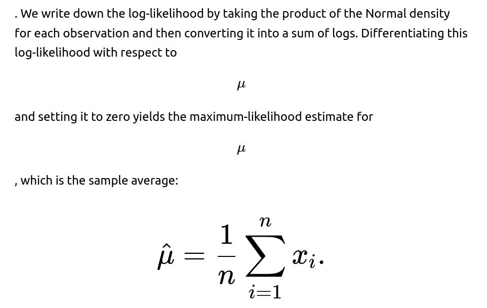
First, we define our model. We assume each observation is drawn from a Normal distribution with an unknown mean and variance. Specifically, we have:


Intuitively, this makes sense: if the data are from a Normal distribution, the best estimate of the true mean is just the average of the values.
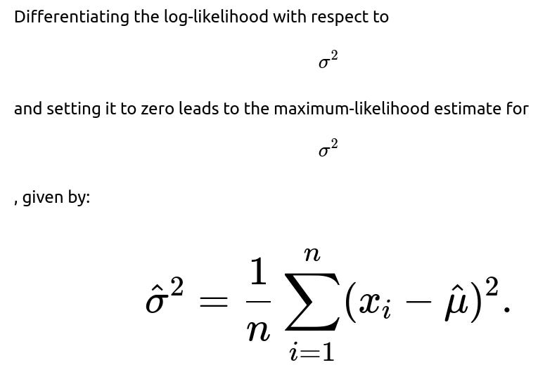
MLE for the Variance


Practical Perspective
These formulas are easy to compute in practice. To implement this in Python, you would typically do:
import numpy as np

X = np.array([...])  # your data
mu_hat = np.mean(X)
sigma2_hat = np.mean((X - mu_hat)**2)
This straightforward procedure is often enough for many practical and theoretical problems when assuming a Normal distribution.
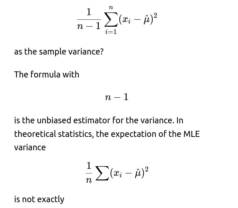
Follow-up question: Unbiased vs. Maximum-Likelihood Variance
Why do we sometimes see

Follow-up question: Effects of Non-Gaussian Data
What if the data are not truly Normal?
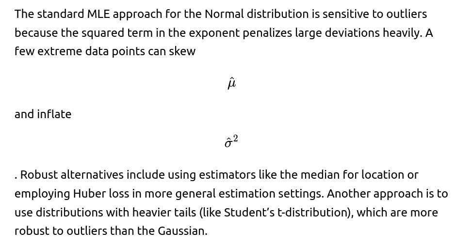
If data deviate substantially from normality, the MLE approach (assuming Gaussianity) may be inappropriate. In reality, an assumption violation can lead to estimates that are suboptimal. Possible solutions include using robust estimators (like median-based approaches or M-estimators), or choosing a model that matches the data distribution more closely (e.g., a Laplace distribution if there are heavier tails).
Follow-up question: Bayesian Estimation Approach


Follow-up question: Numerical Stability in Implementation
How do we avoid numerical issues when computing the log-likelihood for large data?
When the dataset is large or values are large in magnitude, directly computing the product of many probabilities can lead to underflow, and summing many negative log-likelihood components can cause precision difficulties. Strategies to address this include:
Using log probabilities through the entire calculation (which is already done in the log-likelihood).
Potentially leveraging libraries like NumPy or PyTorch that handle summations in a numerically stable manner (such as using
torch.logsumexpor similar functions to reduce underflow issues).Making sure the data are normalized or preprocessed if appropriate.
Follow-up question: Outliers and Robustness
How are outliers handled in this approach?
Follow-up question: When to Prefer the MLE Approach
In what scenarios is the MLE for Gaussian parameters the method of choice?
This approach is ideal when:
We strongly believe the data-generating process is near-Gaussian or the Central Limit Theorem justifies a normal approximation.
We need computational efficiency, as the MLE for Gaussian parameters is very straightforward to compute.
We do not require an unbiased estimator for the variance or we do not mind making minor bias corrections.
In more advanced or nuanced applications, we consider robust statistics, Bayesian models, or more flexible distributions to accommodate real-world data complexities.

Below are additional follow-up questions
How can we derive confidence intervals for the estimated parameters using MLE?

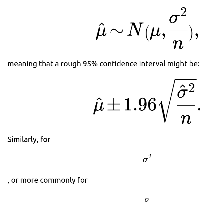
, one can use results on the distribution of the sample variance (though in smaller samples it follows a scaled chi-squared distribution). Potential pitfalls include:
Small sample sizes: The large-sample normal approximation may not hold well. In that case, one might rely on exact distributions or bootstrap methods for more accurate intervals.
Violation of normality: If the data are not truly Gaussian, confidence intervals derived this way can be misleading.

What is the relationship between Maximum Likelihood Estimation and the Method of Moments?
The method of moments (MoM) matches sample moments (like sample mean, sample variance, etc.) to their theoretical counterparts. For a normal distribution, the first two sample moments (mean and variance) turn out to match exactly the MLE solutions:

A subtlety arises with other distributions: MLE and method of moments can yield different parameter estimates. The normal case is special in that the two methods coincide. Pitfalls include:
Complex distributions: In some cases, the method of moments may produce parameter estimates that are outside feasible ranges (e.g., negative standard deviations).
Bias: MLE is often simpler to analyze theoretically with well-understood variance properties, while method of moments can be simpler to compute but does not necessarily minimize the negative log-likelihood.

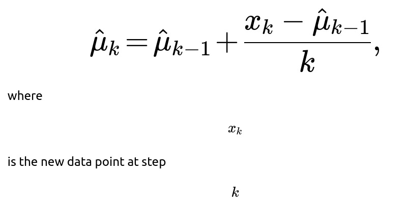
in an online or streaming setting?
In real-world scenarios, data might arrive in a stream, and we want to update our estimates of the mean and variance incrementally without storing all past observations. An online algorithm for updating the mean is:
. For variance, a common approach is to use Welford’s algorithm:
Update the mean with the above formula.
Use the updated mean and old mean to maintain a running sum of squared differences.
The advantage is numerical stability and not needing the entire dataset in memory. Pitfalls include:
Incorrect algorithm implementation: If the online update rule is incorrect, you can systematically bias the variance estimate.
Concept drift: If the underlying distribution changes over time, simply updating might fail to track the new distribution properly. You might need a decay factor or a window-based approach.
What if the data have some known correlation structure among observations?


How do we deal with missing data in computing MLE for a Gaussian distribution?
Real-world datasets often have missing values. If missingness is ignorable (e.g., missing at random), you can use an expectation-maximization (EM) algorithm:

You repeat these steps until convergence. Challenges include:
Non-random missingness: If data are missing systematically, the assumption breaks down and results can be biased.
Convergence: The EM algorithm is guaranteed to increase the likelihood each iteration, but it can converge to a local maximum or be slow in high dimensions.
How does maximum likelihood estimation differ from maximum a posteriori (MAP) estimation in this context?
MAP estimation includes a prior on the parameters. For the Gaussian mean and variance, a conjugate prior is often the Normal-Inverse-Gamma. The MLE results are recovered when the prior is uninformative. The MAP estimate might be written as:

Key differences and pitfalls:
Prior choice: A poorly chosen prior can lead to misleading parameter estimates if it dominates the likelihood.
Small samples: MAP can help regularize estimates in cases where the data are sparse or the dimension is high.
Interpretation: MAP is a single point estimate, while the full Bayesian approach yields a posterior distribution that captures uncertainty more thoroughly.
How do we ensure we actually found a maximum, not a minimum or saddle point, when solving for MLE?
Strictly speaking, setting the gradient of the log-likelihood to zero could yield local maxima, local minima, or saddle points. To confirm you have a maximum:
Second derivative (Hessian) check: Evaluate the Hessian at the critical point. For a univariate parameter, you check that the second derivative is negative at the solution. For multiple parameters, the Hessian matrix should be negative definite.
Convex/concave analysis: For the Gaussian case, the log-likelihood function in terms of

is concave, ensuring that a critical point is a global maximum.
Numerical methods: If implementing iterative methods, you can keep track of function values to confirm they are converging to a maximum.
Pitfalls:
Complex models: For more complicated likelihoods, there can be multiple local maxima. The Gaussian distribution’s log-likelihood is concave in the mean and convex in the variance in a way that typically yields a single global optimum, but this is not guaranteed for other distributions.
Poor initialization: If you are using gradient-based numerical optimization in higher dimensions, starting far from the true solution can lead to slow or inconsistent convergence.


