ML Interview Q Series: Autoencoders: Data Reconstruction for Dimensionality Reduction, Denoising, and Anomaly Detection.

📚 Browse the full ML Interview series here.

Autoencoders: What is an autoencoder? *Describe the structure of an autoencoder (including the encoder and decoder components) and explain how it is trained. What are some practical uses of autoencoders, for example in dimensionality reduction, denoising data, or anomaly detection?*

Overview of Autoencoders

An autoencoder is a neural network architecture designed to learn efficient representations of data (often referred to as latent representations or embeddings) in an unsupervised manner. This is achieved by training the network to reconstruct its own input. The autoencoder typically comprises two primary components called the encoder and the decoder. The encoder compresses or encodes the input into a lower-dimensional space, and the decoder attempts to reconstruct the original input from this compressed representation.

Autoencoders are fundamentally self-supervised because the training target is simply the original input. There is no need for external labels. This self-supervision is powerful for tasks such as dimensionality reduction, denoising, and anomaly detection, among others.

Structure of an Autoencoder

The structure of an autoencoder consists of an encoder, a bottleneck (latent space), and a decoder. The key objective is to minimize the difference between the input and the reconstructed output.

Encoder reduces the dimensionality of the input into a compact representation (the latent vector). Bottleneck is the hidden layer (often smaller in dimension than the original input) that contains a compressed or latent representation of the input. Decoder reconstructs the input from the latent representation.

The network can be fully connected (feed-forward) or can incorporate convolutional, recurrent, or other specialized layers depending on the type of data. For instance, convolutional layers are often used for image inputs, and recurrent layers or Transformers can be used for sequence data like text.

Encoder Component

The encoder is responsible for mapping the original input into a latent representation. Suppose the input is denoted as x. The encoder is a function E(⋅) parameterized by learnable weights, which transform x to a latent vector z. This can be expressed as

z=E(x)

where z is often a vector of reduced dimensionality. The encoder may consist of multiple layers of linear or convolutional transformations combined with nonlinear activation functions such as ReLU, sigmoid, or tanh. The goal is to capture the most salient features of the input in z.

Decoder Component

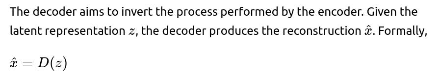
The decoder may mirror the encoder’s structure but in reverse, expanding the latent representation back to the original input dimensionality. If the encoder uses convolutional layers with downsampling, the decoder often uses transposed convolution (or upsampling) to bring the feature maps back to the original input dimensions.

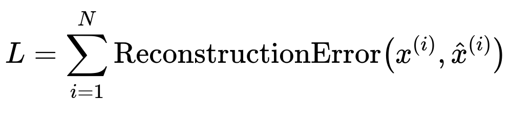
Training an Autoencoder

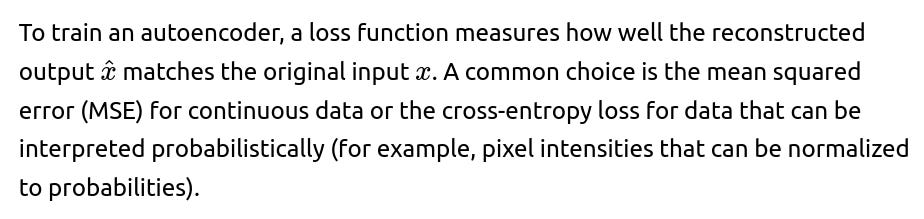
The training process can be expressed as minimizing a reconstruction loss:

Practical Uses of Autoencoders

Autoencoders are used in numerous real-world scenarios. Among the most well-known:

Dimensionality Reduction: Autoencoders can learn low-dimensional representations of high-dimensional data. This can serve as an alternative to traditional methods like Principal Component Analysis (PCA). The latent representation z can be used for downstream tasks such as visualization, clustering, or as input features to other models.

Denoising: A denoising autoencoder is trained with slightly corrupted inputs (e.g., images with added noise) and tasked with reconstructing the clean (noise-free) input. The network learns to remove noise and preserve key features, which is especially helpful in image processing or audio processing pipelines.

Anomaly Detection: An autoencoder trained on normal data learns to reconstruct “typical” examples well. However, if the input significantly deviates from what the network has seen during training, the reconstruction error can be relatively high, signaling the presence of an anomaly. This is useful in fraud detection, industrial sensor data analysis, or any domain where unusual patterns must be flagged.

Other Variants: Variational autoencoders, convolutional autoencoders, and other specialized architectures can tackle problems that require generative modeling, complex feature extraction from image data, or other specialized tasks such as inpainting or super-resolution.

Example Code Snippet in PyTorch

Below is a simple PyTorch example illustrating how one might set up an autoencoder for image data such as MNIST. This version uses fully connected layers and mean squared error as a reconstruction loss:

import torch
import torch.nn as nn
import torch.optim as optim
from torchvision import datasets, transforms

# Simple Feedforward Autoencoder
class Autoencoder(nn.Module):
    def __init__(self, input_dim=784, hidden_dim=64):
        super(Autoencoder, self).__init__()
        # Encoder
        self.encoder = nn.Sequential(
            nn.Linear(input_dim, 256),
            nn.ReLU(True),
            nn.Linear(256, hidden_dim),
            nn.ReLU(True)
        )
        # Decoder
        self.decoder = nn.Sequential(
            nn.Linear(hidden_dim, 256),
            nn.ReLU(True),
            nn.Linear(256, input_dim),
            nn.Sigmoid()  # For MNIST-like data normalized to [0,1]
        )

    def forward(self, x):
        z = self.encoder(x)
        x_recon = self.decoder(z)
        return x_recon

# Data loading and transforms
transform = transforms.Compose([
    transforms.ToTensor(),
    transforms.Lambda(lambda x: x.view(-1)) # Flatten
])
train_dataset = datasets.MNIST(root='./data', train=True, download=True, transform=transform)
train_loader = torch.utils.data.DataLoader(train_dataset, batch_size=128, shuffle=True)

# Initialize model, loss, optimizer
model = Autoencoder()
criterion = nn.MSELoss()
optimizer = optim.Adam(model.parameters(), lr=1e-3)

# Training loop
num_epochs = 5
for epoch in range(num_epochs):
    for data, _ in train_loader:
        # data = batch of images
        reconstruction = model(data)
        loss = criterion(reconstruction, data)

        optimizer.zero_grad()
        loss.backward()
        optimizer.step()

    print(f"Epoch [{epoch+1}/{num_epochs}], Loss: {loss.item():.4f}")

In this simple example, the autoencoder processes batches of MNIST images (reshaped into 784-dimensional vectors). The encoder transforms input images into a lower-dimensional embedding, and the decoder attempts to reconstruct the original images from that embedding. The reconstruction loss is the mean squared error between the original and reconstructed images.

Denoising Example

To transform an ordinary autoencoder into a denoising autoencoder, one can add noise to the input and still use the original clean input as the reconstruction target. In PyTorch, that can be achieved by adding random noise to the input images. The network will learn to produce a clean, denoised version.

One might do:

noisy_data = data + 0.2 * torch.randn_like(data)
reconstruction = model(noisy_data)
loss = criterion(reconstruction, data)

This technique is valuable in real-world settings where data is imperfect or incomplete and can also act as a regularizer that prevents the autoencoder from learning trivial identity mappings.

Follow-up Questions and In-Depth Explanations

Undercomplete vs Overcomplete Autoencoders

An undercomplete autoencoder has a latent space dimension smaller than the input dimension. This enforces a strong compression of the data and helps the model learn salient features that are crucial for reconstruction. By constraining the network capacity (or the size of the latent bottleneck), the network is forced to ignore noise or less important details.

An overcomplete autoencoder has a latent space dimension greater than or equal to the input dimension. This can lead to the risk that the network simply learns to copy the input data to the output without learning meaningful feature representations. Techniques like regularization, sparsity penalties, or denoising objectives are often used to mitigate this risk.

Potential pitfalls: If the autoencoder is overcomplete and not carefully regularized, it might simply memorize the input-output mapping by passing information directly through. This typically does not yield useful compressed representations.

Avoiding the Identity Mapping Problem

A common concern in training autoencoders is the risk that the network learns a trivial function that essentially copies the input to the output without meaningful compression. This risk is especially high if the model architecture has too many parameters or if the latent dimension is not constrained. Approaches to avoid this include:

Adding random noise to inputs (denoising autoencoders). Constraining the bottleneck layer to be narrower. Applying a sparsity penalty on the hidden units so that only a few neurons are active at a time, encouraging more compact representations. Using a contractive autoencoder, which penalizes the sensitivity of the latent representation with respect to input variations. In all these cases, the aim is to force the model to learn robust, generalizable features rather than simply memorizing the input.

Practical Details for Real-World Data

In real-world applications, autoencoders often need to handle large and complex datasets:

Convolutional layers are essential for image data to capture local spatial patterns efficiently. For textual data, it may be beneficial to use recurrent layers (LSTM, GRU) or Transformers in the encoder and decoder components. Regularization and early stopping can be critical to avoid overfitting and ensure that the learned features are generalizable. Batch normalization or layer normalization can be added to stabilize training. Normalization or standardization of input features usually helps. For instance, scaling pixel intensities between 0 and 1 or standardizing input distributions can improve training stability.

Denoising Autoencoders in More Detail

Denoising autoencoders are powerful tools for tasks where the data may be corrupted by noise or other defects. By training on pairs of noisy and clean data, the autoencoder learns a transformation that removes noise. This is of special interest in image processing, speech enhancement, and medical signal processing.

For example, an autoencoder that learns to remove random Gaussian noise from images can be critical for low-light photography or specialized medical imaging devices. After training, the latent representation becomes quite robust to noise, which can also benefit other tasks like classification.

Anomaly Detection with Autoencoders

For anomaly detection, the autoencoder is trained exclusively on “normal” examples. During inference, if the reconstruction error is significantly larger than the typical reconstruction error on normal data, it implies that the network has not seen this type of pattern before, and the data point can be flagged as an anomaly. In practical settings:

It is important to collect representative normal data. If the training data includes mislabeled anomalies, the autoencoder might learn incorrect boundaries of normal behavior. Thresholding on the reconstruction error is typically used to decide which points are anomalies. The threshold can be tuned on a validation set or by domain-specific knowledge. This is widely applied in credit card fraud detection, network intrusion detection, or manufacturing quality control.

Potential Extensions: Variational Autoencoders (VAE)

Variational Autoencoders are a class of generative models that impose a probabilistic framework on the latent space. Instead of mapping an input to a single point in the latent space, VAEs learn a distribution (often Gaussian) over the latent space. This allows the model to generate new data by sampling latent vectors from that learned distribution. Although VAEs fall under the umbrella of autoencoders, they involve additional terms in the loss function, specifically a Kullback–Leibler divergence to regularize the latent distribution.

By introducing a stochastic latent space, VAEs can generate novel data that appears similar to the training data. These are especially interesting for tasks like image synthesis, text generation, or semi-supervised classification.

Practical Issues and Best Practices

Although autoencoders can be extremely powerful, there are some best practices to bear in mind:

Architecture Choice: For image tasks, using convolutional layers in both the encoder and decoder tends to yield better reconstructions than purely dense layers. Latent Dimension: Choosing an appropriate size of the bottleneck is critical. Too small can lead to underfitting, too large can lead to identity mapping or overfitting. Regularization: Sparsity constraints or other forms of regularization often help autoencoders learn more meaningful features rather than simply reconstructing data in a superficial way. Data Preprocessing: Normalizing input data or applying domain-specific transformations is often beneficial for stable training. Training Stability: Monitoring both training and validation reconstruction losses helps identify if overfitting has occurred. Techniques like early stopping or learning rate scheduling can improve generalization.

Handling Highly Imbalanced Data

In some real-world applications, especially anomaly detection, the dataset is highly imbalanced (normal events vastly outnumber anomalies). Since the autoencoder is generally trained only on normal data, it is critical to ensure that normal data is well-represented and varied enough to capture different “typical” scenarios. If the normal data is not diverse, the model may fail to recognize real normal patterns outside of its training distribution, or it might mistakenly identify them as anomalies.

Data augmentation or carefully curated sample collection can help mitigate this problem. If anomalies are partially available, semi-supervised approaches or specialized architecture modifications might further improve detection capabilities.

Handling Non-Stationary Data

When data distribution changes over time (e.g., concept drift), the autoencoder trained on past data might no longer reconstruct the present data effectively. One approach is to retrain or fine-tune the model periodically on more recent data. Another is to employ online learning methods that update the model continuously.

---

Below are additional follow-up questions

How do autoencoders handle multi-modal data (e.g., images, text, audio) simultaneously?

When dealing with multi-modal data, an autoencoder must effectively learn representations that capture the salient features across different data types, each of which may have unique statistical properties. A common strategy is to design modality-specific encoders and decoders for each data modality while sharing a joint latent space. For instance, one could have a convolutional encoder for images, a recurrent (LSTM/GRU) encoder for text, and a 1D convolution or a Transformer-based encoder for audio. These modality-specific encoders map their inputs into a shared latent representation, which the decoders then use to reconstruct each original modality.

Pitfalls and edge cases: If one modality dominates (e.g., a large number of images vs. fewer text samples), the autoencoder might bias its representations toward the dominant modality. Balancing or weighting the loss across modalities is crucial to ensure no single modality overwhelms the learning process. Multi-modal alignment can be challenging if there’s no direct one-to-one pairing between modalities (e.g., missing some audio samples for an image-text pair). In such cases, specialized techniques or partial reconstruction losses can help handle missing modalities. Latency and computational overhead can become significant because each modality might require different architecture types. Careful design and resource management become key in large-scale, real-world deployments.

How can we interpret or visualize the latent representations learned by an autoencoder?

Interpreting latent representations often involves dimensionality reduction and visualization techniques such as t-SNE or UMAP. Even though these are themselves dimension-reduction methods, they can give insights into how data clusters in the autoencoder’s latent space. One can also probe the latent space by perturbing specific dimensions and observing how the output reconstruction changes, effectively gauging which latent variables control which aspects of the data.

Pitfalls and edge cases: Latent spaces can be high-dimensional. Reducing them to 2D or 3D for visualization can lose information, so any conclusions drawn must be tempered with caution. It’s possible that different dimensions in the latent space do not correspond to neat semantic concepts. The representations might be entangled, making it hard to map them onto human-interpretable axes.

What are some strategies to measure the success of an autoencoder beyond the standard reconstruction loss?

While reconstruction loss (like MSE or cross-entropy) is a primary metric, other strategies can be considered depending on the use case: Embedding utility: Evaluate how well the latent representation performs on a downstream supervised task (e.g., classification accuracy). Clustering metrics: If the latent space is intended for clustering, measure cluster quality with metrics like silhouette score or Davies–Bouldin index. Perceptual metrics: For image data, a perceptual loss or Structural Similarity Index Measure (SSIM) can be more aligned with human perception than pixel-wise error. Task-specific criteria: In denoising tasks, one might look at SNR improvements. In anomaly detection, metrics such as precision/recall or AUROC on anomaly labels may be more relevant.

Pitfalls and edge cases: Optimizing only for reconstruction error can lead to an autoencoder that memorizes data without learning genuinely useful features, especially for overcomplete architectures. Applying too many metrics simultaneously can be confusing if they conflict. Clear definition of the end goal is critical.

When might a simpler dimensionality reduction technique (like PCA) be preferred over a more complex autoencoder?

PCA is fast, has a closed-form solution, and is easy to interpret in terms of variance explained. If the data is relatively small or if linear transformations suffice, PCA (or other linear methods) may be perfectly adequate.

Pitfalls and edge cases: If the data manifold is highly nonlinear, PCA may be insufficient, and an autoencoder could reveal more complex embeddings. Overlooking this can hurt performance in tasks that rely on capturing intricate patterns. PCA scales poorly with extremely large datasets in terms of memory usage. Some incremental variants exist, but training an autoencoder incrementally (via mini-batches) might actually be easier for large-scale data.

How can we handle discrete data (e.g., text tokens) with autoencoders?

For text tokens, a common approach is to embed each token into a continuous vector space (via word embeddings or learnable embeddings for subword tokens). An encoder (often based on RNN, CNN, or Transformers) processes these embeddings to produce a latent representation. The decoder must then convert the latent representation back into discrete tokens, typically via a softmax output layer at each step or a more advanced beam search approach if the sequence is long.

Pitfalls and edge cases: Decoding discrete tokens often requires a language-model-like structure in the decoder, which adds complexity. The autoencoder might memorize exact sequences instead of learning generalizable language features if the dataset isn’t large enough. Text can be highly variable in length. Handling variable-length inputs may require attention-based mechanisms or LSTM states, which increases training complexity. Padding and masking must be carefully managed.

What strategies can we use to tune hyperparameters in autoencoder training?

Hyperparameter tuning can be approached with: Grid or Random Search: Brute force or random combinations of layer sizes, learning rates, batch sizes, etc. Bayesian Optimization: More sophisticated searching can converge faster to good hyperparameters. Automated Tools: Libraries like Optuna or Ray Tune can manage large-scale experiments efficiently. Domain-Informed Constraints: For instance, limiting the latent dimension to approximate known degrees of freedom in the data can reduce the search space.

Pitfalls and edge cases: Overfitting can mask which hyperparameters are genuinely best. Regular monitoring on a validation set is crucial. The interactions between learning rate and network capacity can be non-trivial. A large network might demand a lower learning rate or stronger regularization. Hyperparameter tuning in autoencoders can be time-consuming if the dataset is large. Maintaining a robust strategy for logging and comparing different runs is essential to avoid confusion.

How do we scale or distribute training for large autoencoders across multiple GPUs or machines?

Scaling can be done through data parallelism, where each GPU processes a different mini-batch of data, and gradients are averaged before an update step. More advanced methods include model parallelism, splitting the network architecture across devices (e.g., the encoder on one set of GPUs, the decoder on another). Distributed frameworks in PyTorch or TensorFlow can facilitate multi-machine setups.

Pitfalls and edge cases: Synchronizing parameters over large numbers of workers can become a bottleneck. Techniques like gradient compression or asynchronous updates might help but can introduce convergence complexities. Large batch sizes can change training dynamics and potentially require retuning of the learning rate or scheduling. If the batch size is too large, the model may converge to poorer minima or suffer from generalization issues.

How do we handle concept drift or non-stationary data streams with autoencoders?

In a streaming scenario, the data distribution can change over time. An autoencoder trained on past data might become stale or exhibit high reconstruction error on new distributions. Online learning or incremental training can be employed, where parameters are updated continuously with new data. Alternatively, one can periodically retrain or fine-tune the autoencoder with the most recent samples.

Pitfalls and edge cases: If drift is gradual, incremental updates might suffice. If drift is sudden and severe, the model might need to reset or drastically adjust its parameters to accommodate the new distribution. Maintaining a buffer of representative past data is essential if the model must also continue to perform on older distributions (e.g., catastrophic forgetting can occur if only the latest data is used).

How do adversarial autoencoders differ from standard or variational autoencoders?

Adversarial autoencoders (AAEs) incorporate a discriminator network to match the latent code distribution to a prior distribution (e.g., Gaussian). The autoencoder tries to encode inputs in a way that “fools” the discriminator into thinking the latent codes come from the chosen prior. This adversarial training encourages structured latent distributions, much like a VAE but without explicit KL divergence.

Pitfalls and edge cases: Adversarial training can be unstable, requiring careful balancing of the autoencoder and discriminator learning rates and capacities. Mode collapse can occur if the discriminator gets too strong or too weak relative to the encoder-decoder. Architectural choices—such as how to structure the discriminator and how to incorporate reconstruction loss—can have a large impact on results.

What steps can we take if an autoencoder produces blurry or poor-quality reconstructions (particularly for images)?

Blurry reconstructions often indicate that the network is averaging over variations in the data. Potential remedies include: Increasing capacity or adding skip connections (like in U-Net style architectures) that preserve high-frequency information. Using perceptual or feature matching losses (e.g., matching feature maps in a pre-trained network like VGG). Ensuring the model is not overly regularized, which can lead to high bias and underfitting.

Pitfalls and edge cases: Over-increasing the capacity can risk overfitting, especially if the training data is limited. Using complex losses such as perceptual losses can make training unstable if the learning rate is not tuned carefully.

Are there situations where autoencoders are not a good fit, potentially hurting performance or interpretability?

Autoencoders may not be ideal when: You simply need a linear dimensionality reduction and the data is small—PCA can be faster, easier to interpret, and sufficient. You require high interpretability of features. Autoencoder latent dimensions are abstract and might not map to easily explainable features. The data does not need reconstruction. If the only goal is classification and the label is well-defined, a supervised approach with a well-architected network might outperform the extra step of learning an autoencoder.

Pitfalls and edge cases: In some regulated industries (e.g., finance, healthcare), black-box embeddings might not pass interpretability requirements, limiting autoencoders’ utility. Autoencoders can be heavy computationally. If resources are constrained, a simpler method might yield a better cost-benefit ratio.

How do we incorporate domain knowledge into autoencoder-based pipelines for specialized tasks?

Domain knowledge can inform architecture design (e.g., known symmetries or invariances), specialized layers, and the choice of loss functions. For instance, if certain frequency components matter more in an audio signal, the model can incorporate wavelet-based or spectrogram-based transformations before encoding. Similarly, in a medical context, known tissue structures might drive specialized convolutional kernels or multi-stage training where parts of the body are learned separately.

Pitfalls and edge cases: Injecting incorrect domain assumptions can degrade performance. Collaboration with domain experts is crucial. Complex domain-specific modifications can make training harder to debug and tune, especially if libraries aren’t readily available for specialized transformations.

What unique concerns arise when applying autoencoders to time-series data, such as sensor or financial data?

Time-series data has temporal dependencies and often requires specialized recurrent or Transformer-based architectures. The bottleneck must capture temporal dynamics rather than just static features. Additionally, data might have seasonality, trends, or sudden spikes that complicate reconstruction.

Pitfalls and edge cases: Misalignment in time steps can occur if data streams arrive at different frequencies or have missing timestamps. Overly simplistic models that ignore temporal context can produce poor reconstructions or fail to capture leading or lagging indicators in the data. If the data is non-stationary, the autoencoder’s reconstruction quality may degrade quickly without periodic retraining or drift management.

How do we combine autoencoders with downstream tasks (e.g., classification) while preserving reconstruction fidelity?

A common approach is to train a multi-task model. One head of the network focuses on reconstruction, while another head branches from the latent representation for classification or regression. The total loss is a weighted sum of reconstruction loss and task-specific loss.

Pitfalls and edge cases: Balancing the two objectives is non-trivial. If reconstruction is given too much weight, the latent space might not be discriminative enough for classification. If classification dominates, the autoencoder might ignore reconstruction fidelity. Domain-specific considerations for the classification task might conflict with ideal reconstruction. Regular experimentation with weighting is often necessary.

How do we handle memory constraints or limited computational resources while training deep autoencoders on large datasets?

Memory constraints can be addressed by: Using smaller batch sizes or gradient checkpointing to reduce peak GPU memory usage. Adopting a shallow architecture or leveraging techniques like knowledge distillation to compress a larger model into a smaller one. Streaming data in small chunks (e.g., using PyTorch’s IterableDataset) so not all data resides in memory at once.

Pitfalls and edge cases: Excessively small batch sizes can hurt gradient estimation quality, leading to training instability. Checkpointing can slow down training because it re-computes certain intermediate activations during the backward pass. Distilling an autoencoder is trickier than a supervised model because the objective is reconstruction, and specialized teacher-student setups may be needed.

What about using autoencoders for partial or incomplete data? Are there specialized strategies or architectures?

For incomplete data, one approach is to mask missing parts and train the autoencoder to reconstruct the full input. Another is to use dedicated architectures like Masked Autoencoders (MAE) that specifically learn to predict missing tokens/patches from visible context. In structured data, one might have a multi-branch encoder that processes known features and tries to reconstruct all features, treating missing ones as targets.

Pitfalls and edge cases: If a large fraction of data is missing, the model might struggle to learn a meaningful embedding without specialized handling of missingness (imputation, dedicated masks, or specialized loss). Inconsistent patterns of missing data across samples can degrade reconstruction performance unless the architecture explicitly accounts for it.

How can we make autoencoder latent features more interpretable to domain experts?

One possible approach is to impose additional constraints or structure on the latent space—sparse autoencoders, grouped latent units corresponding to domain components, or semi-supervised approaches that tie certain latent dimensions to known labels. Another strategy is a “bottleneck interpretability” method where each latent dimension is explicitly tied to a specific aspect of the data, although this often requires domain-specific assumptions or partial supervision signals.

Pitfalls and edge cases: Overly restricting the latent space might reduce reconstruction fidelity if the constraints are unrealistic. There’s always a trade-off between interpretability and flexibility. Using partial labels or domain groupings can require labor-intensive data annotation or domain knowledge, which might not always be feasible at scale.

What difference does it make if we turn an autoencoder into a generative model (e.g., Variational Autoencoder or Adversarial Autoencoder)?

By introducing a probabilistic or adversarial objective, we move beyond pure reconstruction to also shaping the latent distribution. This allows for sampling new data points from the latent space, effectively enabling generative capabilities: Variational Autoencoder: Adds a KL divergence term that enforces a Gaussian latent space, providing a direct way to sample novel points. Adversarial Autoencoder: Uses a discriminator to match latent codes to a prior distribution, creating a flexible generative framework.

Pitfalls and edge cases: Generative training can produce blurred or less diverse samples if hyperparameters aren’t well-tuned. Balancing the adversarial or KL term with the reconstruction loss requires careful experimentation, or the network might degenerate to either ignoring the prior or ignoring reconstruction quality.

How can we do domain adaptation or transfer learning with autoencoders from one domain to another?

One strategy is to train an autoencoder on a large source dataset and then fine-tune either the entire network or just the decoder on the target domain data. Alternatively, domain adaptation can involve matching latent distributions across domains (e.g., using adversarial techniques to make the latent representations domain-invariant).

Pitfalls and edge cases: If the source and target domains are drastically different, the shared autoencoder might not transfer well. Negative transfer can occur if features learned for the source domain are misleading for the target domain. Some tasks require specialized fine-tuning of only certain layers. For instance, keeping early convolutional layers fixed if they capture generic features, but re-learning deeper layers or the decoder to adapt to domain-specific structures.

When an autoencoder is used as a feature extractor for a classification pipeline, how do we ensure that the learned features are relevant?

Some practitioners pre-train an autoencoder and then use the latent representations as inputs to a classifier. Relevance is boosted by: Providing a task-related regularization or a small label-based objective during autoencoder training. This becomes a semi-supervised approach, nudging latent features toward discriminative aspects. Checking classification metrics (precision, recall, F1-score) on a validation set to see if the features significantly outperform a baseline.

Pitfalls and edge cases: There’s no guarantee the unsupervised features are aligned with the specific classification labels. This can lead to suboptimal performance compared to purely supervised learning, especially if large labeled data is available. Excessive focusing on reconstruction might capture non-discriminative details, diluting the representation needed for classification.

Is it possible to use autoencoders for data augmentation, and how might that be done effectively?

Autoencoders can be used to generate new synthetic samples by sampling points in the latent space and decoding them. For tasks like anomaly detection or classification with limited data, these synthetic samples might enhance performance.

Pitfalls and edge cases: Vanilla autoencoders don’t necessarily learn a smooth latent space suitable for sampling, especially if the autoencoder doesn’t impose a well-defined prior distribution. VAEs or adversarial autoencoders are more suitable for generative augmentation. Generated samples might be too similar to existing data (poor coverage of the true data distribution) or contain artifacts that hamper model training.

In implementing autoencoders in practice, what are common coding mistakes (e.g., dimension mismatch, forgetting certain normalizations)?

Common pitfalls include: Dimension mismatch: Failing to reshape the data correctly between encoder and decoder, especially with convolutions vs. flatten operations. Not applying the same data preprocessing or normalization at inference time as during training. This leads to inconsistent reconstruction performance. Forgetting to detach certain tensors when computing auxiliary losses in more complex autoencoder variants, which can lead to unexpected gradient flows.

Pitfalls and edge cases: Small mistakes in code (e.g., using the incorrect activation or forgetting a final layer’s shape) can cause cryptic errors or degrade performance significantly. Mismanagement of GPU vs CPU data, especially in multi-GPU setups, can lead to out-of-memory errors or silent performance bottlenecks. Careless initialization or no initialization strategy can hinder convergence, leading to vanishing or exploding gradients.