
ML Interview Q Series: Average Time Between Fair Die Rolls: A Geometric Distribution Approach.

Browse all the Probability Interview Questions here.
30. Suppose you roll a fair die n times, where n is very large. What is the average time between occurrences of a given number?
Understanding The Core Probability Concept
In this problem, we consider a fair 6-sided die that is rolled many times. We want to know the “average time between occurrences of a given number,” such as the face “3,” or any other specific face we choose. By “time between occurrences,” we typically mean the expected number of rolls we wait from one appearance of that face until the next time it appears again.
One classical way to see it is that each roll is an independent trial. The probability of rolling a specific face (like “3”) on any given roll is 1/6. The random variable that describes how many rolls occur until we first see a particular number (or until we see it again) follows the geometric distribution in a discrete sense. For a fair die, the probability that it takes exactly k rolls to see the target face for the first time is

The expected value of X, which is the average number of rolls needed to get one success (rolling the target face), is
where p = 1/6 in our fair die case. Therefore,
E[X]=6
This shows that, on average, we wait 6 rolls to see the target face. Equivalently, the “time between” consecutive appearances of the given face is 6, on average.
Hence, the simple, concise answer is that the average time between occurrences of a given number on a fair 6-sided die is 6.
Detailed Reasoning Without Using Numbered Points
We consider each die roll as an independent Bernoulli trial with probability p of success (where “success” is rolling the chosen face). Because of the independence, the number of trials between successive appearances of the chosen face is geometrically distributed.
The geometric distribution quantifies how many Bernoulli trials we expect until we get the first success. In our case, it also measures the gap (in rolls) between consecutive appearances of our target face. Since p = 1/6, the expected value of a geometrically distributed random variable with parameter p is 1/p = 6.
This result holds true regardless of how large n is, as soon as “n is large enough” that we can speak of repeated occurrences. Even over a finite but sizable number of rolls, the average gap between occurrences will be close to 6 if we gather enough data.
Because the question specifically says n is very large, we are effectively invoking the law of large numbers. As we roll the die many times, the observed average gap between rolls that show our chosen number approaches 6.
Illustrative Python Example
import random

def average_time_between_occurrences(num_rolls=10_000_000):
    target_face = 3
    last_occurrence = None
    gaps = []

    for i in range(num_rolls):
        roll = random.randint(1, 6)
        if roll == target_face:
            if last_occurrence is not None:
                gap = i - last_occurrence
                gaps.append(gap)
            last_occurrence = i

    # Return the average gap if we have any recorded
    return sum(gaps)/len(gaps) if gaps else None

if __name__ == "__main__":
    print(average_time_between_occurrences())
In practice, if you run the above code with a large number of rolls, you should see the output hover around 6, confirming the theoretical result.
Subtleties and Pitfalls
One subtle point is the distinction between the “expected number of rolls until the first occurrence” and the “expected gap between occurrences.” Both cases lead to a geometric distribution with parameter p = 1/6 in a fair die scenario. This is because each new roll is an independent trial and the chance that the target number appears on any given roll remains 1/6.
Another subtlety is that in actual finite experiments, especially if n is not extremely large, you will see variations around the theoretical average. But as n becomes large, the average gap converges to 6 due to the law of large numbers.
Potential Real-World Relevance
Even though the question is framed in the context of rolling a die, this type of reasoning generalizes to many real-world processes where events occur with some fixed probability p each “trial.” The average interval or gap between occurrences in these Bernoulli processes is 1/p, which is a foundation for modeling waiting times, system reliability, and other probability-driven phenomena.
What if the die were biased?
If the die were biased in such a way that a particular face comes up with probability p, the expected time between consecutive occurrences of that face would be 1/p. For instance, if a die is biased and a certain face appears 40% of the time (p = 0.4), the average gap between successive appearances of that face would be 1/0.4 = 2.5.
How can we see this in terms of the law of large numbers?
In the limit of many rolls, the fraction of rolls that show the target face should converge to p = 1/6. Thus out of n rolls, roughly n/6 of them show the target face. Therefore, the ratio of total rolls to total occurrences (which is essentially the average gap size) goes to 6 in the fair die case. This is a direct application of the law of large numbers.
What if we consider the variance or higher moments?
The variance of the number of trials until the first success in a geometric distribution with parameter p is (1 - p) / p². For the fair die with p = 1/6,
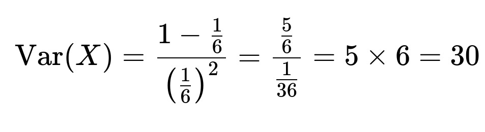
So beyond just the average gap of 6, the variance is 30. This can be useful to understand how spread out the waiting times can be. In finite practice, it’s possible to see consecutive appearances quite close or quite far apart, but on average, the gap is 6.
How can we formally connect this to Markov chains or renewal processes?
Each roll can be viewed as a Markov chain state with some memoryless property. However, an even simpler framework is renewal theory, where “renewals” happen each time we roll the target face. The times between renewals follow a geometric distribution (in a discrete setting). Renewal processes help model events occurring over time where each inter-arrival time is an independent identically distributed random variable.
Could we approach this using expected values from first principles without referencing the geometric distribution?
Yes, we can attempt a direct approach by considering the probability that a gap is exactly k and summing k times that probability, but that derivation leads to the same result: 6. A simpler approach is by acknowledging that each roll has probability 1/6 for the target face. Hence one can reason directly that if each outcome is equally likely, in the long run you see one target face per every six rolls.
What might happen if you only record the gaps after a long burn-in period?
In practice, especially for large n, it typically doesn’t matter if you ignore the first partial gap before the first occurrence. As n grows, the contribution of the first partial gap to the overall average becomes negligible. The average gap measured after a long run will still approach 6.
How does this scale with the number of sides on the die?
If instead of a 6-sided die, you had an s-sided die and each side remained equally likely (p = 1/s), then the average time between consecutive occurrences of a specific face would be s. This generalizes straightforwardly and is consistent with the expectation formula for a geometric random variable with probability p = 1/s.
Once you have answered the main question and offered these deeper discussions, an interviewer might probe your understanding further by asking the next set of questions. Below are more possible follow-ups, together with thorough answers.
How do you reconcile this with the possibility of rolling the same face multiple times in a row?
It can happen that the same face appears consecutively. In some trials you might have zero-gap (i.e., the target face appears on two successive rolls). But the expected gap accounts for all possibilities, including short gaps of 1 roll and longer gaps of 20 or more. The probability distribution still evens out in the long run to an average gap of 6.
Are there practical considerations in large-scale simulations of random events?
Yes, one important consideration is the quality of the random number generator. If you are simulating dice rolls in a computer, you rely on pseudorandom generation. For extremely large n, subtle biases in the random generator could affect empirical measurements. However, typical modern pseudorandom libraries are robust, and you will see results in line with theoretical expectations (like an average gap of 6).
How does this problem tie into machine learning or large-scale data analysis?
Within machine learning or data science contexts, you often sample from distributions or gather events with some probability. Understanding these waiting time distributions or the concept of the reciprocal of event probability (1/p) helps design experiments, interpret repeated events, and model processes that generate data. For example, in online recommendation systems or marketing funnels, the “average time to an event” could be analogous to an “average number of user sessions until a purchase.” The mathematics is the same, except that the probability p may not be 1/6 but could be based on complex user behaviors. Still, 1/p remains the expected waiting time.
When linking it back to real-world data, you might see slight deviations because real-world events often do not precisely follow independent Bernoulli assumptions. That’s where more advanced approaches or additional modeling is needed.
Below are additional follow-up questions
What if we only record occurrences of the target number once we have already seen it at least once?
In some practical scenarios, you might decide to begin measuring gaps only after the first time the target number appears. This can arise if you start your experiment upon seeing the first success or due to instrumentation constraints, such as only logging data once a sensor first triggers. The key question is whether this changes the average time between subsequent occurrences.
For a geometric distribution with probability of success p=1/6 the average gap between occurrences of the target number does not change, even if you “discard” the partial gap before the first occurrence. The reason is that each new roll of the die is memoryless: no matter what happened in the past, the probability of seeing the target number on the next roll remains 1/6. The expected gap after you have seen the target once is still 1/p=6.
A subtle pitfall here is that people sometimes assume the first gap from the start might bias the subsequent intervals. However, due to the memoryless property, ignoring the partial gap up to the first occurrence does not affect the distribution of future intervals. The only scenario where it might matter is when the process is not truly memoryless. For example, if the probability of rolling a certain face could change over time, or if your data collection starts at a moment that is not stationary. But in the ideal setting of a fair die with independent, identical trials, the expected gap after the first success is still 6.
How does the answer change if we simultaneously track multiple different faces?
Sometimes you want to track more than one “target” face, for instance, looking for either 3 or 5 on a fair die. In that case, you have two events you consider “success.” The probability of rolling either 3 or 5 on a fair die is 2/6=1/3. If you are interested in the average gap between occurrences of “3 or 5,” then by the same geometric distribution logic, p=1/3, which yields an expected gap of 1/p=3 rolls.
However, it is trickier if you specifically want to track the times between occurrences of 3 only, and 5 only, in the same sequence. The average gap for 3 alone would still be 6, and the same for 5 alone. But if your question changes to “when do we next see either 3 or 5,” it is 1/(1/3)=3.
A subtlety arises when you want to measure the gap between 3’s given that we might see 5’s in between. It does not alter the expected time specifically for 3, but it does change how we interpret “an occurrence we care about.” Understanding precisely what your “success” event is (maybe “3,” maybe “3 or 5”) is crucial to correct expectation calculations. A pitfall is mixing up different success criteria in the same measurement process, which can lead to incorrect or confusing results if not clearly delineated.
How might correlated rolls affect the average time between occurrences?
The classical result that the average gap is 6 relies heavily on the assumption of independence. If rolls become correlated—for example, if there is a physical defect causing the die to stick on certain faces more frequently if it just landed on them—then the probability of the target face might not be a constant 1/6 each time. In that case, the distribution of waiting times would deviate from the geometric distribution.
If, hypothetically, the chance of rolling a 3 after you just rolled a 3 is higher (positive autocorrelation), then consecutive 3s may cluster, lowering the observed average gap for 3. Alternatively, if rolling a 3 once makes it less likely to appear on the immediate next roll (negative autocorrelation), the average gap might increase above 6.
In real-world physical dice, correlation is usually negligible unless the die is severely biased or there’s a mechanical process forcing repeated faces. Another subtle point can be overly simplified random number generators in simulations, which might inject mild correlation. In practice, strong correlation in dice is unusual but can occur in other domains (like sensor data, network requests, or user event logs). In those correlated contexts, you must adjust your theoretical expectation for average waiting times because the memoryless geometric assumption no longer holds.
How do we handle rolling multiple dice at once for each “trial” and looking for a specific face?
Consider a scenario where each “trial” is actually rolling M dice in parallel. You still want to know the average “time” until you see your target number appear on at least one die among those M dice. If each die is fair and the event is “at least one of the dice lands on 3,” the probability of success in a single trial becomes:
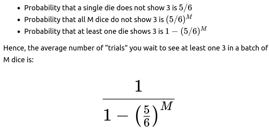
If you define “time” strictly as the number of trials (where each trial is an M-dice roll), that is the expected number of such multi-die trials until success. If you define “time” as the total number of individual dice rolled, then in each trial you effectively roll M dice, so you might multiply the expected trial count by M.
An edge case arises if you only look for “exactly one 3 among M dice,” or “3 appears at least twice,” and so on. Each variant changes the probability of success for a single trial. A pitfall is mixing up the definition of one “trial” (roll M dice once) with the definition of one “roll” (roll a single die). Carefully define your random variable and measure your gap accordingly.
Does the geometric distribution approach still work if the probability of rolling the target face changes over time?
In real-world systems, probabilities can shift dynamically. Suppose at the start the probability of rolling a 3 is 1/6, but after some time, you swap to a different die with a slightly different bias. Or the environment changes so that your original assumption no longer holds. Then the process is not strictly a single-parameter geometric distribution with a fixed p.

How would we approach this problem if the “die rolls” were continuous random events?
Sometimes waiting times are modeled in continuous time. For instance, if events are happening at times drawn from a Poisson process with rate λ, the waiting time between events follows an exponential distribution with mean 1/λ. A fair die scenario in discrete time is analogous to a Bernoulli process, which leads to a geometric distribution.
If you asked, “On average, how long until a certain continuous-time event occurs?” and each event had probability p within a short interval, you could end up bridging to a Poisson process if each discrete time step is infinitesimally small. The key difference is that in continuous-time processes, you might have an exponential distribution for waiting times. In discrete-time processes (like rolling dice), you have a geometric distribution. Both share the memoryless property if the underlying process is stationary (Poisson in continuous time, Bernoulli in discrete time). A pitfall is mixing continuous-time assumptions with discrete data or vice versa. The concept is similar, but the exact formulas differ (E[exponential]=1/λ vs. E[geometric]=1/p).
Could the “time between occurrences” question be tackled by Markov chain states?
A single die roll can be considered a Markov chain with 6 states (one state per face outcome). However, for the question of “time between occurrences of face i,” you often reduce it to a simpler one-step memoryless process. The Markov chain perspective can be overkill unless we incorporate more complicated dynamics, such as transitions that depend on previous states. In that scenario, each state could carry memory that influences the probability of landing on each face next.

How can partial or missing data affect the estimate of average time between occurrences?
In real data collection, you might have incomplete logs: some rolls are unobserved, or the system fails to record certain events. This missing data can bias the observed average gap. For instance, if half the time you fail to log the occurrence, you could overestimate the true gaps. The question becomes how to correct your analysis to account for missing data.
One approach is to model the chance of “seeing” a roll as a Bernoulli process independent of the actual face outcome. If the missingness is random with respect to the face value, you may still estimate unbiasedly by adjusting the observed frequencies. However, if there is systematic bias—for example, your sensor fails more often when the die shows 3—then your estimates of p and the resulting gap times are no longer straightforward to correct.
A pitfall is assuming you can just scale everything by the fraction of missing data. If the missingness is correlated with the event of interest, you must model that correlation or risk severely incorrect estimates. This is especially tricky when the fraction of missing data is large or when you have no knowledge of the missingness mechanism. In such real-world scenarios, advanced missing data techniques or additional instrumentation may be needed to recover a reliable estimate of the true waiting times.
How does the central limit theorem help us understand variability in the measured average gap?
When you perform an experiment of n rolls and measure the average gap between occurrences of the target face, you essentially collect a large number of i.i.d. “waiting times.” Each of these waiting times has mean 6 and variance 30 for the fair die. If you measure the sample mean gap across many occurrences, the central limit theorem tells you that as the number of occurrences grows, the distribution of the sample mean around the true mean (6) becomes approximately normal with a standard deviation shrinking at the rate ParseError: KaTeX parse error: Expected 'EOF', got '_' at position 21: …rt{\text{number_̲of_occurrences}….

How might the time between occurrences be estimated in an online (streaming) setting?
In a streaming setting, you do not have all n rolls in advance; instead, new rolls come in continuously. You might want an online algorithm to estimate the average gap. One practical approach is to maintain running statistics: each time the target face appears, compute the gap from the previous occurrence, update a running sum of gap values, and increment the count of observed gaps.
A simple incremental algorithm would look like this in Python:
count_gaps = 0
sum_gaps = 0
last_occurrence_index = None
roll_index = 0

def update_estimate(roll_value):
    global count_gaps, sum_gaps, last_occurrence_index, roll_index

    if roll_value == 3:  # Suppose 3 is our target
        if last_occurrence_index is not None:
            gap = roll_index - last_occurrence_index
            sum_gaps += gap
            count_gaps += 1
        last_occurrence_index = roll_index
    roll_index += 1

def get_average_gap():
    if count_gaps == 0:
        return None
    return sum_gaps / count_gaps
This online approach updates the average gap in real time. One subtlety is that if the stream changes properties over time (e.g., the probability of 3 changes or the dice become biased), your older gap measurements might not be representative of the new reality. Hence, you might wish to implement a weighted or “forgetting” factor to place more emphasis on recent gaps. Another edge case is the possibility of extremely long intervals without the target face, which may skew your estimates if you stop collecting data too soon. In a truly indefinite stream, you simply keep refining your estimate as more occurrences happen.
Are there scenarios where the “average time between occurrences” is not the best metric?
The mean gap of 6 is certainly a key statistic, but in some situations, other properties might be more relevant. For example:
• Median gap might be interesting if you want to know a typical gap that’s robust to outliers. The geometric distribution can have high variance, meaning occasionally very long streaks of not seeing the target face. • Confidence intervals or percentile bounds (such as a 95th percentile) might matter if your system requires certain performance guarantees like “at most 20 rolls pass without seeing 3, with 95% probability.” • Inter-arrival times might be better summarized by a complete distribution rather than just the mean.
In some real-world tasks, extreme values can matter more than the mean. For instance, if we are talking about critical failures in a system, the tail of the distribution can highlight risks. A pitfall is focusing on the average alone when what you really need is a fuller picture of the distribution.
How do we handle a scenario where each roll takes a varying amount of “time,” instead of being identical, instantaneous trials?
Typically, we imagine each die roll as a single, uniform time step. But in real experiments, you might find that rolling and reading the outcome can vary in duration. If the time cost for each roll is random or changes systematically (e.g., the next roll might take longer if the previous roll was a 6, or due to mechanical constraints), then you have two layers of randomness: (1) whether the target face appears, and (2) how long each roll takes.
You could model it as a renewal reward process: each “trial” has a random reward (the time cost) plus an indicator for success or failure. The question “How long, on average, in real time does it take until we see the target face?” then becomes a mixture of the geometric distribution (for the count of trials) and the distribution of each trial’s duration. If each trial’s duration is i.i.d. with mean T, and the probability of success in each trial is p=1/6, then on average, you need 1/p trials. So the average total time is:

For a fair die, that would be 6×E[trial duration]. One subtlety arises if the time distribution per roll depends on whether you succeed or fail or on the outcome of the roll. Then you cannot simply multiply. You must compute the unconditional expectation by carefully summing or integrating over all possible durations weighted by success probabilities. A pitfall is simplifying incorrectly when time per roll is correlated with the result.
Does the initial state or “warm-up period” matter if we are rolling indefinitely?
When n is extremely large, the fraction of rolls you perform before seeing the target face for the first time becomes negligible, so the system is effectively “stationary” for the vast majority of the experiment. In the limit, the law of large numbers ensures the observed frequency of the target face converges to p=1/6, and thus the observed mean gap converges to 6.
However, if you are in a short-run scenario with small n, the initial phase can indeed have an outsized impact on your measured average gap. For example, if you get “unlucky” at the beginning and it takes many rolls to see the target the first time, that might shift your overall average gap over the smaller sample. Another subtlety is if your system starts in a known or unknown “initial state” that might bias the early rolls. Once again, for a fair die, we typically assume each roll is i.i.d. from the start, so there is no “initial condition” effect. But in real systems or more complex processes, you often have a distinct initialization that might skew early waiting times. The pitfall is ignoring the possibility of a non-stationary start if you only have limited data. Over large n, that issue usually dissipates.
How can we check empirically that the gap is indeed 6 in a real or simulated experiment?
A straightforward empirical check is to:
Simulate or perform a large number of rolls (or gather real data).
Each time the target face appears, record the index of that roll.
Compute the differences between consecutive indices to get a list of gaps.
Calculate the mean of those gap values.
Compare that mean to 6.
In Python, you could do something like:
import random

def check_gap(num_rolls=1_000_000, target_face=3):
    last_occurrence = None
    gaps = []
    for i in range(num_rolls):
        roll = random.randint(1, 6)
        if roll == target_face:
            if last_occurrence is not None:
                gaps.append(i - last_occurrence)
            last_occurrence = i

    if gaps:
        return sum(gaps)/len(gaps)
    else:
        return None

print(check_gap())
Over many runs with num_rolls in the millions, you should see an empirical average close to 6. You can also plot a histogram of the gaps to see the geometric-like distribution. One real-world pitfall is underestimating the amount of data needed to get stable estimates, especially because the geometric distribution has a relatively heavy tail. If you only roll the die a few dozen times, you might see large deviations from 6. Another subtlety is ensuring your pseudo-random generator is good quality to avoid hidden correlation or biases.
Does the law of large numbers guarantee we will get exactly 6, or might there be deviations?
The law of large numbers states that as n grows, the sample average of i.i.d. random variables converges to the true expectation. However, it does not guarantee that you will get exactly 6 or that you will see 6 in any finite experiment. Rather, it tells you that as the number of occurrences goes to infinity, the sample average gap is increasingly likely to be very close to 6.
In finite experiments, you can have the phenomenon of “runs” or “clusters” where the same face appears repeatedly in short order, driving the observed gap below 6 for a while. You can also have lengthy dry spells. Over the long term, these fluctuations average out. A pitfall is to treat the “6” as a deterministic guarantee in any short-run scenario. Instead, it is only the long-run expected value. For engineering or risk management, you might need to factor in the probability of unusually large gaps if they can cause real-world issues (e.g., “the system cannot tolerate going 30 or more rolls without the target face”).
Is there a closed-form expression for the distribution of the sum of multiple geometric random variables?
Sometimes you care about the total number of rolls until the target face appears k times, which is a negative binomial distribution. Specifically, if each success occurs with probability p=1/6, and you want k occurrences, the distribution for how many rolls are needed to reach k successes is negative binomial. The expected total rolls to get k occurrences of the target face is:

so for p=1/6 and k successes, it becomes 6k. This is effectively the sum of k independent geometric random variables, each with mean 1/p=6. A pitfall is mixing up the average waiting time for a single occurrence with the total number of rolls needed to see multiple occurrences. Another subtlety is that the negative binomial distribution has a known closed-form probability mass function, but the sum-of-geometric perspective is typically how it is derived. If you want to know the distribution of sums or the variance, you can use the known formulas from negative binomial. This is important if you need the exact probability that it takes more than a certain number of rolls to see k occurrences.
How does this reasoning extend to a die with S sides?
Finally, if you generalize to a fair die with S sides (instead of 6) and you pick one face to track, the probability of rolling that face on a single roll is 1/S. The average gap between occurrences remains the reciprocal of that probability:
For a fair 10-sided die, it would be 10. For a fair 20-sided die, it would be 20, and so on. The same geometric distribution logic holds as long as each side is equally likely on every roll and the rolls are independent. An edge case is if the die is not fair (say a 10-sided die with different probabilities for each face), in which case you simply invert the probability of the target face to get the expected gap. Another subtlety arises if you choose multiple faces or more complex events, but the fundamental principle—“the expected waiting time is 1/p for an event with probability p”—still applies.