
ML Interview Q Series: Balancing Classes: Resampling, Weighting, and SMOTE for Imbalanced Data Classification.
📚 Browse the full ML Interview series here.
Imbalanced Dataset: Your training dataset for a classification problem is highly imbalanced (say 95% of samples belong to one class and 5% to another). What problems can this cause for a model’s learning and evaluation? Describe techniques to handle imbalanced data, such as resampling (oversampling or undersampling), class weight adjustments, or generating synthetic data (SMOTE).
Thinking Summary (concise): The core issue with imbalanced data is that the model can become biased toward predicting the majority class, as optimizing for overall accuracy may ignore the minority class. We need approaches such as specialized metrics (precision, recall, F1-score, AUC), rebalancing the dataset (oversampling, undersampling, SMOTE), or adjusting the training process (class weighting, focal loss) to remedy this. Below is an extensive, in-depth explanation that follows the instructions.
Problems Caused by Imbalanced Data One major issue is that a naive model can learn to predict the dominant class almost exclusively. If your training set is 95% majority class and 5% minority class, a simple model that labels every sample as majority might reach 95% accuracy, even though it is clearly useless for capturing the minority class. This leads to over-optimistic performance estimates if you only look at accuracy. Another problem is that standard loss functions (like cross-entropy) might not penalize misclassification of the minority class heavily enough, which further biases the model to favor the majority class. Additionally, metrics such as accuracy and even unweighted loss may fail to detect whether the minority class is recognized properly.
A subtle challenge arises when your minority class is truly rare, like fraud detection or disease diagnosis. The cost of misclassifying a minority-class example (a fraudulent transaction missed or a positive disease test incorrectly labeled negative) can be extremely high. Traditional training that focuses on overall accuracy does not incorporate that cost asymmetry. As a result, performance for the minority class is often poor without proper handling of the imbalance.
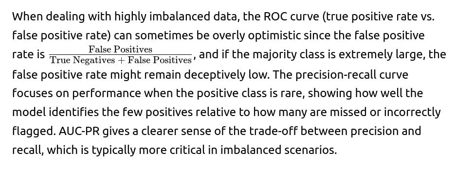
Why Evaluation Becomes Tricky Evaluation is also misleading if you rely solely on metrics like accuracy. Instead, you should examine precision, recall, F1-score, AUC-PR (Area Under Precision-Recall Curve), or AUC-ROC (Area Under the Receiver Operating Characteristic Curve). These metrics give a clearer sense of how well the model handles the minority class:
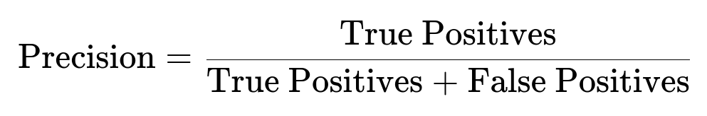
The above measures the proportion of predicted positives that are truly correct. In a heavily imbalanced scenario, a small number of false positives can drastically lower precision.
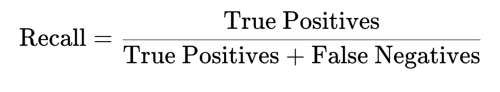
This measures the proportion of actual positives that the model successfully captured. In many real-world imbalanced situations (like medical diagnosis), recall for the minority class is critical.
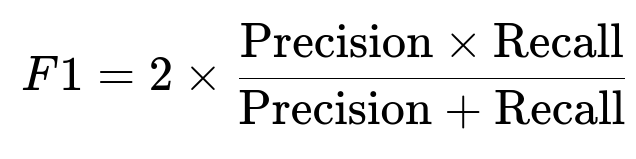
F1 is the harmonic mean of precision and recall, useful when you want a combined measure of precision and recall, especially if you care equally about both.
Properly selecting and interpreting these metrics is essential for a realistic evaluation of your model’s performance when dealing with imbalanced data.
Resampling Approaches Resampling modifies the distribution of classes in your training set so it becomes more balanced. The main categories are oversampling the minority class or undersampling the majority class.
Oversampling. This involves taking additional copies of the minority class samples (random oversampling) or generating synthetic samples based on the distribution of the minority class. A simple approach is random oversampling: you randomly replicate minority examples until the classes are balanced. However, random oversampling can lead to overfitting because the same minority data points appear multiple times.
Undersampling. This involves randomly removing samples from the majority class. It directly reduces dataset size on the majority side to rebalance. However, undersampling may discard a lot of potentially valuable data from the majority class, risking underfitting or loss of important majority-class variety.
Balancing oversampling and undersampling. Often, you might combine both: you remove some samples from the majority class and replicate or generate some new minority samples, attempting to achieve a balanced mix with minimal overfitting or lost information.
Generating Synthetic Data (SMOTE and Variants) The Synthetic Minority Oversampling TEchnique (SMOTE) is a popular method to create synthetic minority examples. SMOTE works by interpolating between existing minority samples. Suppose you have a minority sample in feature space and you pick one of its nearest neighbors (also from the minority class). SMOTE creates a new sample by picking a point along the line segment between these two points. In code:
import numpy as np

def smote_sample(x_i, x_j, random_state=None):
    """
    x_i, x_j are vectors from minority class
    returns a synthetic sample along the line between x_i and x_j
    """
    if random_state is not None:
        np.random.seed(random_state)
    lam = np.random.rand()  # random number [0, 1]
    return x_i + lam * (x_j - x_i)
This approach yields more "unique" data points than naive replication and can help the model generalize better. However, you must be careful because synthetic points might not always be realistic. For example, if the minority class distribution is multi-modal, interpolating blindly can produce samples that do not belong to any real sub-distribution. Extensions of SMOTE (like Borderline-SMOTE or SMOTEENN) are designed to mitigate such problems.
Class Weight Adjustments Another widely used method is to adjust class weights. Many libraries, such as scikit-learn, PyTorch, and TensorFlow, allow you to weight the loss function differently for each class so that mistakes on minority-class samples incur higher penalty. For example, if you have class 0 (majority) with 95% samples and class 1 (minority) with 5% samples, you can set the weighting in inverse proportion to class frequency:
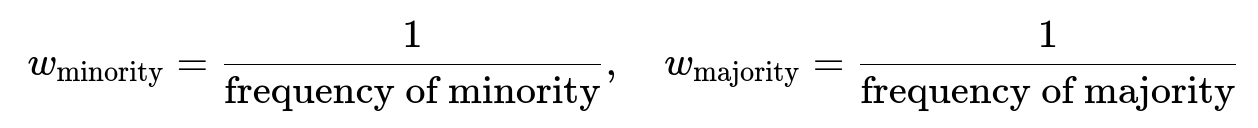
This forces the model to pay more attention to minority-class errors without changing the data distribution itself. Adjusting class weights is useful in neural network frameworks:
import torch
import torch.nn as nn

# Suppose we have a binary classification with 95:5 ratio
# For convenience, define weights inversely proportional to these frequencies
class_weights = torch.tensor([0.05, 0.95])  # This can be tuned or done automatically
criterion = nn.CrossEntropyLoss(weight=class_weights)
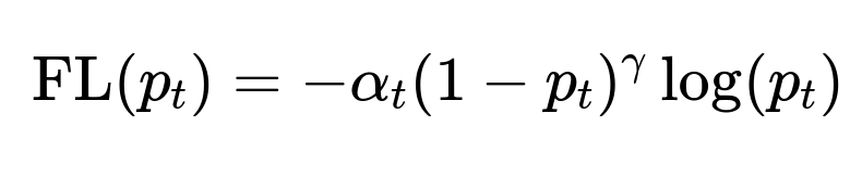
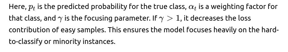
Focal Loss A specialized variation of weighted cross-entropy is focal loss. It was introduced for object detection tasks (particularly in the RetinaNet paper) to handle foreground-background class imbalance, but it is generally helpful for imbalanced classification. Focal loss applies a modulating factor to the cross-entropy to reduce the relative loss for well-classified samples and focus more on hard, misclassified examples:
Practical Implementation Details When deciding how to handle imbalance:
Choose the right evaluation metric. Do not rely solely on accuracy. Use metrics like F1-score, AUC-PR, or ROC-AUC, focusing on the minority class performance.
Try class weighting first. It is simple, does not alter your dataset, and is straightforward to implement in most machine learning libraries.
If you have a small minority dataset and can afford the potential risk of overfitting, try oversampling or SMOTE. But watch for the risk of creating synthetic data that does not reflect real minority patterns.
If you have sufficient data in the majority class, consider undersampling carefully. You do not want to lose essential majority patterns, so random undersampling might be a last resort unless the majority class is extremely large and redundant.
Often, you combine class weighting with oversampling. There is no universal formula; you must experiment with cross-validation to find the best combination.
Monitoring Overfitting and Generalization Overfitting is a risk, especially if you replicate minority examples repeatedly (or generate synthetic samples in a naive way). To mitigate overfitting:
Use cross-validation or hold-out sets that maintain class proportions. Evaluate using metrics like AUC, precision-recall, or F1 for the minority class.
Monitor training and validation loss curves (or other relevant metrics) to detect whether the model is memorizing re-sampled points.
Consider advanced data augmentation for the minority class if relevant (e.g., for images, you could apply transformations that preserve class identity).
Potential Follow-up Questions and Answers
How should you choose between oversampling and undersampling in practice?
Both approaches have trade-offs. Oversampling can lead to overfitting the minority data if done naively (like simple random oversampling), but it preserves all the majority-class information. Undersampling is simpler in that it avoids artificially creating new samples, but it risks losing significant information about the majority class. In practice, a balanced approach is often used:
You might do partial undersampling to remove a large chunk of redundant majority data. Then you apply SMOTE or another oversampling technique to the minority class to avoid overfitting. Experimentation is crucial. You can track how each method affects your validation metrics and pick the one that yields robust performance without excessive overfitting.
Why might simple accuracy be misleading in highly imbalanced tasks, and which metrics are best?
When one class dominates, predicting everything as that class might achieve very high accuracy but fail entirely at identifying the minority class. Accuracy does not capture the trade-off between false positives and false negatives when classes are imbalanced. Better metrics include precision, recall, F1-score, and especially the area under the precision-recall curve (AUC-PR). These metrics do not become artificially inflated just because the majority class is easy to predict. Precision-recall metrics highlight how well the model is identifying the minority class.
Can you give an example of how to handle class weights in PyTorch or TensorFlow for an imbalanced classification problem?
Yes. In PyTorch, you would typically create a tensor of weights, one per class, then pass that to the loss function. For example:
import torch
import torch.nn as nn
from torch.utils.data import DataLoader

# Suppose we have a dataset with an imbalanced distribution
# Let's compute class weights inversely proportional to their frequencies
# freq = [num_class_0, num_class_1]
freq = [950, 50]  # Example: 1000 data samples with 95:5 ratio
weights_for_loss = [sum(freq)/f for f in freq]
weights_for_loss = torch.tensor(weights_for_loss, dtype=torch.float)

criterion = nn.CrossEntropyLoss(weight=weights_for_loss)

# Then define your model, optimizer, etc., as usual
# model = ...
# optimizer = ...

# Train loop
# for data, target in dataloader:
#     optimizer.zero_grad()
#     output = model(data)
#     loss = criterion(output, target)
#     loss.backward()
#     optimizer.step()
In TensorFlow (Keras), you can set class_weight when you call model.fit. For instance:
class_weights_dict = {0: sum(freq)/freq[0], 1: sum(freq)/freq[1]}

model.fit(
    X_train,
    y_train,
    epochs=10,
    batch_size=32,
    class_weight=class_weights_dict
)
This ensures that the gradient updates pay more attention to errors on the minority class.
How does SMOTE differ from just random oversampling?
Random oversampling simply replicates existing minority samples, leading to exact copies of the same data points. This does not introduce new patterns and risks overfitting. SMOTE (Synthetic Minority Oversampling TEchnique) creates new samples by interpolating between existing minority samples. This results in more diverse synthetic examples that capture variations, potentially improving generalization. However, SMOTE can still produce samples that may not align perfectly with the underlying data distribution if the minority class is heterogeneous, so it is important to verify that SMOTE’s assumptions hold in your dataset.
What if you have many features, some of which are high dimensional? Does SMOTE still work?
SMOTE generally can work in high-dimensional spaces, but interpolation becomes trickier because of the curse of dimensionality. Distances in high-dimensional space can be less meaningful, and finding truly “close” neighbors might be challenging. In such scenarios, advanced variants like SMOTE for high-dimensional data, or specialized dimensionality reduction before oversampling, might help. You could consider principal component analysis or autoencoder-based feature reduction, then apply SMOTE in a lower-dimensional space to generate more plausible minority examples.
If I only have a small minority dataset, can I instead gather more real data or generate synthetic data in a more domain-aware manner?
Yes, that is often preferable. When possible, collecting additional real samples from the minority class is the gold standard. Synthetic data generation methods (like SMOTE) are best used as a fallback when data collection is difficult, expensive, or impossible. In some domains, advanced domain-specific augmentation strategies are superior. For instance, in image classification, you might use transformations like flipping, rotation, or color jittering to expand your minority class. In text classification, you might apply synonym replacement or back-translation. The key is to produce augmented samples that remain faithful to the label.
Are there ensemble methods tailored for imbalanced data?
Yes, there are techniques like Balanced Random Forest, EasyEnsemble, or SMOTEBoost. In Balanced Random Forest, each tree in the ensemble is trained on a balanced bootstrapped sample (undersampled from the majority class and possibly oversampled from the minority). EasyEnsemble trains multiple classifiers on different subsets of the majority class combined with the entire minority class, then aggregates the results. SMOTEBoost applies SMOTE at each iteration of boosting to create a new balanced dataset for training the next weak learner. These ensemble strategies often produce robust performance on imbalanced datasets because they combine rebalanced training subsets and ensemble diversity.
How do you monitor training progress when using resampling or class weighting?
You must monitor metrics that reveal minority-class performance. Keep track of recall, precision, F1-score, or AUC-PR for the minority class. Plot these metrics over epochs. Pay special attention to whether the minority-class recall is improving at the expense of precision or vice versa, and see if the majority-class performance is tanking (which could be undesirable if it matters for your application). Cross-validation is extremely useful in ensuring your oversampling or undersampling approach generalizes rather than overfits to a particular data split.
What if the imbalance is extreme, for example 99.9% to 0.1%?
When imbalance is that severe, typical resampling might not be enough. You may need specialized anomaly detection approaches (if the minority samples truly represent anomalies), advanced hierarchical modeling, or one-class classification methods. Gathering more data from the minority class is often crucial, as model-based approaches alone might not suffice. Alternatively, you could adopt a cost-sensitive approach where misclassifications of the minority class incur a substantially higher penalty. You can also attempt multi-stage detection processes: a first-stage filter identifies “potential” minority cases, followed by a more specialized classifier. This architecture can focus capacity on a tiny subset where the minority is more likely to occur.
How do we decide on the threshold for classification in an imbalanced setting?
Even after training, the typical 0.5 probability threshold may not be optimal for minority-class detection. You can adjust the decision threshold based on your desired precision-recall trade-off. A common practice is to use a validation or hold-out set and compute precision-recall or F1 metrics across different thresholds:
import numpy as np
from sklearn.metrics import precision_score, recall_score, f1_score

def best_threshold(y_true, y_prob):
    thresholds = np.linspace(0, 1, 101)
    best_f1 = 0
    best_t = 0
    for t in thresholds:
        y_pred = (y_prob >= t).astype(int)
        f1 = f1_score(y_true, y_pred)
        if f1 > best_f1:
            best_f1 = f1
            best_t = t
    return best_t, best_f1
This way, you select the threshold that maximizes the metric relevant to your application (e.g., F1, or a weighted version of precision and recall, or even a custom cost function).
Could you elaborate on when to use precision-recall AUC instead of ROC AUC?
If my minority class is not just smaller but also more diverse, does oversampling still help?
Yes, oversampling can help, but you must be careful. If your minority class is very diverse, naive SMOTE might create unrealistic interpolations that do not match the true subclusters in your minority class. In this case, you might need cluster-based oversampling: first cluster your minority samples (e.g., via k-means), then oversample within each cluster to avoid mixing different minority modes. Alternatively, more advanced synthetic data generation methods might be needed to handle the wide range of variations in the minority data.
If I incorporate class weights, do I still need to do oversampling or undersampling?
Class weights and rebalancing techniques can be used separately or in combination. Sometimes just using class weights is enough. However, if the minority class is extremely small, you might still benefit from oversampling to provide the model with more minority examples during training. Realistically, you will often try a range of strategies—class weighting alone, SMOTE alone, class weighting + SMOTE, or other sophisticated approaches. The best method is chosen by comparing validation performance under your target metrics.
What are the main pitfalls or edge cases in resampling?
One key pitfall is overfitting, especially if your dataset is not large overall. Random oversampling or SMOTE might lead the model to memorize a few minority samples. Another pitfall is losing majority-class diversity with undersampling, especially in high-variance situations where the majority class covers a large portion of the feature space. A third pitfall is creating unrealistic synthetic data with SMOTE that misleads the model. Finally, resampling might change the distribution in a way that no longer reflects real-world conditions. If your real-world distribution is truly 95:5, artificially balancing it to 50:50 might affect how well the model calibrates probabilities, so you often have to calibrate or adjust the decision threshold later.
Could you provide some code illustrating a practical training loop for an imbalanced dataset with oversampling in PyTorch?
Here is an example that uses a PyTorch Dataset, along with a simple WeightedRandomSampler to oversample minority classes:
import torch
from torch.utils.data import Dataset, DataLoader, WeightedRandomSampler
import torch.nn as nn
import torch.optim as optim

class MyImbalancedDataset(Dataset):
    def __init__(self, features, labels):
        self.features = features
        self.labels = labels

    def __len__(self):
        return len(self.labels)

    def __getitem__(self, idx):
        x = self.features[idx]
        y = self.labels[idx]
        return x, y

# Suppose we have data with features in X, and labels in y
X = torch.randn(1000, 20)  # 1000 samples, 20 features
y = torch.cat([torch.zeros(950, dtype=torch.long), torch.ones(50, dtype=torch.long)])

dataset = MyImbalancedDataset(X, y)

# Compute class counts
class_counts = [torch.sum(y == 0).item(), torch.sum(y == 1).item()]
weights_per_class = [1.0 / c for c in class_counts]
weights = [weights_per_class[label] for label in y]

sampler = WeightedRandomSampler(weights, num_samples=len(weights), replacement=True)
loader = DataLoader(dataset, batch_size=32, sampler=sampler)

model = nn.Sequential(nn.Linear(20, 10), nn.ReLU(), nn.Linear(10, 2))
criterion = nn.CrossEntropyLoss()
optimizer = optim.Adam(model.parameters(), lr=1e-3)

for epoch in range(10):
    model.train()
    for batch_x, batch_y in loader:
        optimizer.zero_grad()
        outputs = model(batch_x)
        loss = criterion(outputs, batch_y)
        loss.backward()
        optimizer.step()
    # Evaluate, log metrics, etc.
Here, WeightedRandomSampler effectively oversamples the minority class by sampling them more often. This approach keeps your original dataset intact but modifies how batches are drawn. After training, you would carefully evaluate using a separate validation or test set that has the true distribution.
In summary, what is the general process when dealing with highly imbalanced data?
You first analyze the dataset to understand the class distribution and the cost of errors. Then you choose proper evaluation metrics that highlight performance on the minority class. You can adjust your training process via class weighting, resampling (oversampling, undersampling, SMOTE), or specialized losses such as focal loss. You carefully verify performance using cross-validation and the right metrics, possibly adjusting classification thresholds for the best balance of precision and recall. You also remain vigilant about overfitting and ensuring your final model generalizes to real-world data distributions.
Below are additional follow-up questions
How can data augmentation be applied to textual data in an imbalanced classification setting?
Textual data presents unique challenges for resampling and data augmentation. Unlike image data, where you can apply flips or rotations while preserving meaning, text requires transformations that maintain semantic integrity. One approach is synonym replacement, where words in the minority samples are replaced with synonyms from a lexical resource. Another method is back-translation, where you translate minority-class sentences into another language and then translate them back to the original language, hoping to preserve semantics but add small variations in word choice and phrasing. For example:
You can use a pipeline where you translate English text into French, then translate the French back into English. This yields additional data that is close in meaning to the original minority sample yet not identical. Another technique is random insertion or deletion of words, but you must ensure the label remains unchanged. These domain-aware augmentation strategies help avoid the simplistic duplication that leads to overfitting.
Pitfalls arise if the augmentation drastically changes the text’s meaning. You must monitor the quality of augmented data and ensure labels are still correct. For instance, a sentiment classification example might accidentally transform a negative statement into a less negative one via back-translation. Automatic synonyms can be misleading when words have multiple senses. Thus, augmenting textual data is highly domain-specific; human review or careful validation is often necessary to avoid generating contradictory or noisy samples.
When is cost-sensitive learning a more suitable approach than resampling?
Cost-sensitive learning is especially useful when misclassifying minority samples has a quantifiable financial or risk-based cost that is significantly higher than misclassifying majority samples. Unlike resampling, which manipulates the dataset distribution, cost-sensitive methods directly modify the learning objective by imposing higher penalties for mistakes on certain classes. This approach is more suitable when:
You have a well-calibrated notion of how costly each type of error is. For example, in fraud detection or medical diagnosis, the cost of missing a positive case can be explicitly higher than a false alarm. You want to preserve the actual distribution of your data to maintain probability calibration. Resampling might artificially distort the distribution, while cost-sensitive learning retains the real data proportions but makes minority errors more expensive. You have multiple classes or a complex cost matrix that does not lend itself well to a simple oversampling/undersampling strategy.
A potential challenge is tuning the cost parameters. If costs are too high for the minority class, the model might overfit those samples and produce too many false positives. Conversely, if the cost is set too low, minority instances still might not get enough attention. Cross-validation or domain knowledge is crucial in determining the appropriate cost matrix.
How do you handle multi-class scenarios where multiple classes have significantly different frequencies, not just a single minority?
In many real-world problems, you might have multiple classes with varying frequencies. For instance, you might have five classes, each representing a different category of user behavior, and some classes might have 60% of the samples while others have only 2%. Traditional binary imbalance methods like SMOTE or weighted cross-entropy can be generalized to multi-class settings. You can:
Assign class weights inversely proportional to the frequency of each class. That means each class gets a weight that is the total number of samples divided by the number of samples for that class. This forces the loss function to pay more attention to the rarer classes. Apply SMOTE or other synthetic data generation techniques on a per-class basis. However, you must carefully handle how synthetic data is generated when multiple minority classes exist, especially if some minority classes are outliers or have overlapping distributions. Use specialized multi-class oversampling or undersampling strategies that treat each class individually while trying not to oversample the extremely small classes to the point of overfitting.
Edge cases can arise if some classes are extremely rare, such that only a handful of samples exist. Oversampling or SMOTE in such classes may produce unrealistic samples if there is not enough original diversity. You might need more specialized solutions or additional data collection focused on those rare classes. Ensuring you evaluate each class separately (via confusion matrices and per-class metrics) is critical to measure progress fairly.
How do you handle changes in the data distribution over time when the minority class proportion shifts?
Real-world systems often experience concept drift. For instance, in fraud detection, fraudsters adapt, causing both the overall incidence of fraud and the nature of fraudulent transactions to change. In time-dependent scenarios, the minority class proportion might go from 5% to 10% or drop from 5% to 1%. You must adapt your models accordingly:
Implement online or incremental learning, where the model updates continuously as new data arrives. This lets you adjust to new minority-class proportions without retraining from scratch on the entire historical dataset. Use a sliding window or weighting scheme that prioritizes recent data. If the minority proportion changes drastically, historical data might become less representative of the current distribution. By focusing the model more on recent samples, you can handle the shift more gracefully. Continuously monitor performance metrics, especially minority-class recall. If performance degrades, investigate whether the class ratio changed or if the nature of the minority examples has evolved.
A subtle pitfall is that older synthetic data or oversampling strategies might no longer reflect the new distribution or the new minority-class characteristics. Ensuring your data pipelines and model architecture can handle dynamic rebalancing is crucial in production systems that see frequent distribution shifts.
How can you deal with the situation where the majority class itself may be composed of multiple distinct sub-groups with different distributions?
It is possible that the majority class is not a single homogeneous class but rather an aggregate of different sub-populations. If you simply undersample the majority class indiscriminately, you may lose critical sub-group representation. This becomes problematic if your ultimate goal is not just to identify the minority class but also to understand or classify different segments within the majority class.
One strategy is cluster-based undersampling. You cluster the majority class samples into sub-groups, then undersample proportionally within each cluster to preserve diversity. Alternatively, you could use methods like SMOTE for the minority class while ensuring that each sub-group in the majority class remains sufficiently represented. Another approach might be to treat each sub-group as a separate “class,” then consolidate them for final classification if it is logically consistent with your task. The main pitfall is inadvertently discarding essential variety from the majority, leading to an underrepresented region in feature space that the model cannot learn accurately.
How do you perform probability calibration in an imbalanced dataset?
Calibration refers to ensuring that a predicted probability truly reflects the likelihood of being in the positive (or minority) class. In highly imbalanced data, models can become poorly calibrated because they rarely see positive examples and might output probabilities that do not align well with real-world frequencies. You can address this by:
Using temperature scaling or Platt scaling on a validation set that reflects the real imbalance. For instance, you can take the model’s logits or raw probabilities, learn a temperature parameter or a logistic function that adjusts the predicted probabilities to match the observed frequencies in your validation data. Employing calibration curves, such as reliability diagrams, to visualize the mismatch between predicted probabilities and actual outcomes. If the curve indicates systematic under- or over-confidence, you adjust accordingly via a post-processing step. Continuing to evaluate with metrics like Brier score, which is sensitive to proper calibration. A good model for imbalanced data might have a strong recall but still exhibit poor probability calibration, so separate calibration checks are essential.
A tricky scenario emerges if your training procedure uses resampling or heavy class weighting. The distribution seen by the model differs from the real-world distribution. After the model is trained, you must recalibrate on data that has the true distribution. Otherwise, your model might systematically overestimate the minority probability. This additional calibration step is critical for real-world decision-making.
How can extremely large training datasets with relatively few minority samples be handled more efficiently?
When you have a massive dataset with billions of majority samples and only thousands or tens of thousands of minority samples, training on the entire dataset is computationally expensive, and random undersampling might still leave you with a large majority portion. Consider these strategies:
Targeted sampling or stratified sampling, where you ensure each training batch contains all minority samples or a proportionally higher number of minority samples, while randomly sampling a smaller fraction of majority examples. This technique can dramatically reduce training costs without losing too much major-class diversity. Use hashing or approximate nearest-neighbor methods to identify which majority samples are most relevant or “close” to minority samples, then focus training on those regions of feature space rather than the entire majority distribution. This local approach can preserve the most critical majority examples for distinguishing from minority examples. Consider an offline method to cluster or compress majority data. You represent each cluster by a centroid plus representative samples. This cluster-based summarization can drastically reduce the scale of majority data while retaining the core variability.
In practice, the main pitfall is ensuring that you still preserve enough majority-class variety to avoid a biased or incomplete representation. A large dataset might contain many subpopulations of the majority class, and failing to include them can harm generalization. Careful cross-validation helps detect whether your sampling strategy has excluded important parts of the majority distribution.
How can domain-specific knowledge shape decisions about rebalancing techniques?
In many fields—medical diagnostics, cybersecurity, manufacturing quality control—domain expertise can inform which approaches to use. For example, a medical expert might point out that certain transformations of minority cases (e.g., certain data augmentations or synthetic generation) do not make sense if they create biologically implausible samples. Similarly, in cybersecurity, labeling anomalies as minority might require specialized synthetic generation methods that preserve key threat indicators.
Domain knowledge can guide which features should not be altered during SMOTE or other synthetic generation. It can also suggest cost structures for cost-sensitive learning; if missing a critical anomaly leads to significant financial loss or security breaches, the cost matrix must reflect that. A potential pitfall is ignoring domain constraints, resulting in a well-performing model on rebalanced data that fails in real scenarios because it learned patterns from augmented samples that could never occur in the real environment.
What if the minority class is inherently noisy or contains uncertain labels?
In imbalanced datasets, minority labels can sometimes be incomplete or noisily labeled, especially in scenarios like anomaly detection where labeling anomalies requires significant effort or subjective judgment. The smaller the class, the greater the relative impact of label noise. If a fraction of minority examples are mislabeled, oversampling or SMOTE can proliferate these noisy labels, severely undermining model performance.
One solution is to implement robust label-cleaning or label-refinement processes before any oversampling. Techniques like active learning can help identify mislabeled minority samples by showing uncertain samples to experts for re-checking. You can also adopt semi-supervised or weakly supervised learning if some minority labels are uncertain, using multiple confidence levels or data-driven estimates of label reliability. A major pitfall is that if you apply SMOTE or replicate mislabeled minority samples without cleaning, the model will learn from incorrect data that are given disproportionate attention.
How do you handle highly imbalanced regression problems?
While most classic imbalance discussions focus on classification, regression tasks can also face an imbalance in target distributions, for example predicting how many days until a rare failure occurs (with many short times to failure and very few extremely long times, or vice versa). Standard oversampling or class weighting does not directly apply because you do not have discrete classes, but you can adapt some ideas:
You might discretize your continuous target into bins (e.g., “very short time,” “short time,” “medium time,” “long time,” “very long time”) if it makes sense in your domain, then treat it as a multi-class imbalanced problem. You can sample more frequently from the region of the target distribution that is underrepresented (for example, extremely rare high values) to ensure the model sees enough examples there. This might involve a custom sampler that picks more samples from the tail of the distribution. Cost-sensitive techniques can be adapted for regression by imposing higher penalties for errors in specific target ranges. This effectively weights the loss function in favor of the rare but critical target range.
A subtle issue is that artificially balancing the target distribution might mislead the model about real-world frequencies. If you do so, you must calibrate or adjust the model’s outputs to reflect real distribution frequencies. Another challenge is that if the rare targets are also inherently more variable, the model might struggle to capture them even with oversampling.
How do you debug a model that yields high recall but very low precision in an imbalanced scenario?
This often happens when you aggressively optimize for minority-class recall by oversampling or heavily weighting the minority class, leading the model to label too many samples as minority. To debug:
Examine the false-positive patterns by identifying where the model is over-predicting minority labels. Check whether those samples are borderline or if there is a systematic pattern of misclassifying a certain subset of majority data. Tune the decision threshold if you are working with probabilistic outputs. A threshold of 0.5 might not be appropriate for your cost structure. Lowering the threshold helps recall but often hurts precision, so you might find a new threshold that balances them better. Review whether your training approach (like SMOTE or cost-sensitive weighting) has gone too far in emphasizing the minority class. Possibly reduce the oversampling ratio or reduce the class weight. Investigate if the minority class is truly that difficult to separate from some portions of the majority class. Domain knowledge can reveal additional features or transformations that better discriminate the two classes.
The primary pitfall is ignoring the real-world impact of false positives. For tasks like disease screening, too many false positives can lead to unnecessary medical tests or costs. In other contexts, such as security alerts, an excess of false alarms can cause alert fatigue. Balancing recall and precision is thus highly domain-specific.
Can we use anomaly detection methods instead of standard classification to handle an imbalanced dataset?
Yes, if the minority class represents anomalies or out-of-distribution patterns (e.g., fraudulent transactions), anomaly detection methods might be more appropriate. These methods often learn what “normal” looks like (based on majority data) and then flag deviations. Traditional supervised approaches rely on labeled examples of both classes, but if the minority class is extremely small or not fully labeled, anomaly detection might be more robust.
Typical anomaly detection algorithms (like One-Class SVM, Isolation Forest, or Autoencoders) do not require balanced data. They focus on identifying points that do not conform to the learned “normal” pattern. The challenge is that if your minority class does not manifest as outliers in feature space, then typical anomaly detection might fail. Another pitfall is that “normal” data could itself be diverse, which can cause many false positives. Hence, anomaly detection is not a universal replacement for dealing with imbalanced data, but it is an option worth exploring in certain use cases.
What special considerations apply if the minority class changes in meaning or definition over time?
Sometimes, the definition of what constitutes the minority class can shift—for example, in spam detection, new forms of spam might arise that do not match historical examples. This introduces not only distributional shift but also concept evolution, where the label itself is redefined. In such cases, you may have to:
Regularly gather new labeled data that reflects the updated minority definition. The model cannot learn what it has never seen. Use transfer learning or incremental learning approaches that allow you to adapt from old definitions to new ones without forgetting previously learned knowledge that might still be partially relevant. Implement a labeling pipeline that can quickly incorporate new or re-labeled minority samples so the model can retrain or fine-tune in near real-time.
A hidden pitfall is clinging to older minority examples that no longer match the current concept. Mixing them into your training data can confuse the model. You might need to depreciate or re-label them if they do not reflect the new definition. Monitoring real-world performance and engaging with domain experts is key whenever the minority class definition is fluid.
Are there hardware or distributed computing considerations for extremely skewed data?
When datasets are enormous and class distributions are skewed, distributed training frameworks (e.g., PySpark, Horovod, or distributed TensorFlow) might be used. In these settings, ensuring a balanced feed across distributed workers becomes challenging. If you undersample or oversample only on a single node, you might not effectively replicate that distribution across the entire cluster. You must consider:
Coordinated resampling or weighting across all workers so each mini-batch seen by each worker maintains the correct ratio of classes. Efficient memory and data-transfer management. Oversampling a tiny class can balloon dataset size, leading to high communication overhead. An alternative is WeightedRandomSampler approaches that do not create new copies, thus reducing data duplication. Fault tolerance and load balancing. If certain workers handle only minority samples and crash, it might skew training further.
These infrastructure-level details become important in large-scale production systems. A common pitfall is inadvertently replicating minority data many times across multiple nodes, potentially compounding the risk of overfitting. Ensuring consistent sampling policies with robust data pipelines is essential for correct distributed training.
How can interpretability methods help confirm that an imbalanced classification model is making sensible decisions?
Interpretability techniques, such as feature importance, SHAP (SHapley Additive exPlanations), or LIME (Local Interpretable Model-agnostic Explanations), can highlight why a model is labeling certain samples as minority class. When dealing with imbalanced data, focusing on minority-class predictions is crucial. You can:
Use local explanation methods (e.g., LIME) on minority-class predictions to see if the model is leveraging meaningful features or if it is picking up spurious correlations. Compare feature importances for minority vs. majority classification to see if the model employs drastically different logic. If you notice bizarre or irrelevant features strongly influencing the prediction, it might indicate the model is overfitting to a small subset of minority samples. Validate domain consistency. If the interpretability methods show the model paying attention to features known to be relevant to the minority condition, that is a good sign the model is learning genuine patterns rather than random noise.
Pitfalls include misinterpreting interpretability results. With highly imbalanced data, the few minority instances might lead to uncertain or unstable importance estimates. Thorough cross-validation and repeated analysis of explanation methods can mitigate these uncertainties.
How do you determine whether your resampling or weighting strategy has truly improved the model beyond random chance?
After applying resampling or weighting, you might see an improvement in recall or F1-score for the minority class. However, you should rigorously check statistical significance. Techniques include:
Bootstrapping your evaluation set or applying repeated cross-validation splits to gather distributional estimates of metrics. This helps confirm the improvement is not due to random variation in how you sampled or partitioned the data. Performing significance tests such as McNemar’s test (for classification tasks) on predictions from different models. Although these tests assume certain distributions, they can indicate whether the performance difference between the baseline model and the rebalanced model is statistically meaningful. Paying attention to business or practical significance. Even if the numeric improvement is statistically significant, is it large enough to matter in real-world usage? For example, if your recall goes from 0.80 to 0.81, that might or might not be a meaningful improvement depending on the context.
A major pitfall is ignoring confidence intervals for your metrics. With a small minority class, your sample size for evaluating minority performance is small, so the variance of your estimates (precision, recall, etc.) can be high. Always ensure you report confidence intervals or standard deviations across multiple runs to get a robust sense of improvement.