ML Interview Q Series: Bayesian Assessment of Content Rater Diligence Using Labeling Data

Jun 03, 2025

Browse all the Probability Interview Questions here.

12. Facebook has a content team that labels pieces of content as spam or not spam. 90% of them are diligent (labeling 20% spam, 80% non-spam), and 10% are non-diligent (labeling 0% spam, 100% non-spam). Assume labels are independent. Given that a rater labeled 4 pieces of content as good (non-spam), what is the probability they are diligent?

Solution Explanation

Bayes' Theorem is generally applied to update the probability of a hypothesis (that a rater is diligent) after observing some evidence (all 4 labeled as non-spam).

To formalize:

Let D = event that a rater is diligent Let ND = event that a rater is non-diligent

P(D) = 0.9 (prior probability that a rater is diligent) P(ND) = 0.1

If someone is diligent, the probability of labeling a single piece of content as non-spam is 0.8. If someone is non-diligent, they label everything non-spam with probability 1.

We observe 4 pieces of content all labeled as non-spam. Denote this event as E. The goal is to find P(D | E), the probability of being diligent given that all 4 items were labeled as non-spam.

Where P(E | D) = (0.8)^4 P(E | ND) = (1)^4 = 1

So:

P(E | D) = 0.8^4 = 0.4096 P(E | ND) = 1

Now substitute:

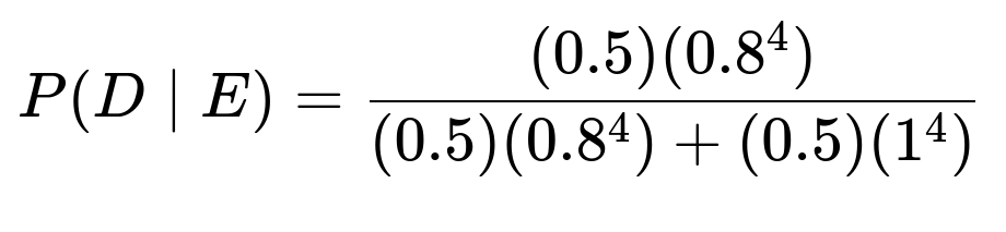
P(D | E) = [0.9 * 0.4096] / [0.9 * 0.4096 + 0.1 * 1]

Numerator = 0.9 * 0.4096 = 0.36864 Denominator = 0.36864 + 0.1 = 0.46864

Final result:

P(D | E) = 0.36864 / 0.46864 ≈ 0.787

Hence, the probability is about 78.7% that the rater is diligent, given they labeled 4 pieces of content as good (non-spam).

Implementation Example in Python

import math

p_dil = 0.9          # Probability rater is diligent
p_non_dil = 0.1      # Probability rater is non-diligent

p_good_if_dil = 0.8
p_good_if_non_dil = 1.0

# All 4 labeled as non-spam
p_all_good_if_dil = p_good_if_dil**4
p_all_good_if_non_dil = p_good_if_non_dil**4

posterior_dil = (p_dil * p_all_good_if_dil) / (p_dil * p_all_good_if_dil + p_non_dil * p_all_good_if_non_dil)
print(posterior_dil)  # ~0.787

Deep Dive into Potential Follow-up Questions

What assumptions are made about independence, and why is that crucial here?

In this setup, we assume each of the 4 labeling events is conditionally independent given whether the rater is diligent or not. That means once we know the rater’s status (diligent vs. non-diligent), the probability distribution of each label does not depend on how the other pieces of content were labeled. This independence assumption is crucial because it lets us multiply the probabilities for each piece of content when computing P(E | D). If dependencies existed (e.g., the rater changes behavior after seeing certain types of content), the calculation would need a more complex joint probability model that incorporates those dependencies.

A subtlety here is that in many real-world labeling tasks, independence can be questionable. A rater’s fatigue, content similarity, or time constraints might cause them to label consistently or inconsistently across multiple items. Yet for a straightforward application of Bayes’ Theorem in an interview or textbook scenario, the conditional independence assumption is very common and simplifies calculations significantly.

How might this result change if the diligent raters also sometimes label spam incorrectly?

If a diligent rater sometimes incorrectly labels spam as non-spam, we would adjust the probability of labeling any piece of content as non-spam. In the original scenario, we assume a single probability (0.8) of labeling content as non-spam for diligent raters. If in a real scenario, “diligent” means a certain accuracy level for both spam and non-spam, one would need a confusion matrix:

Probability of labeling spam as spam
Probability of labeling spam as non-spam
Probability of labeling non-spam as spam
Probability of labeling non-spam as non-spam

In that case, the problem might be more nuanced because the data we see (the 4 pieces labeled as good) could each be spam or not spam in an unknown distribution. The original question effectively simplifies by stating that 20% spam, 80% non-spam labeling is the ratio for a diligent rater, ignoring potential mistakes or differences in the content’s ground truth. If the “20% spam” means the rater is labeling everything with a certain distribution regardless of the true content, the question remains consistent with the stated probabilities. But in a scenario modeling true positives/negatives, you would have to incorporate the underlying distribution of spam vs. not spam as well.

Why does the posterior probability increase as we see repeated evidence of non-spam labeling?

The posterior probability that the rater is diligent increases as they label multiple items as non-spam because the diligent rater has a smaller but still significant probability (0.8) of labeling each item as non-spam. The non-diligent rater, on the other hand, will always label items as non-spam with 100% probability. Intuitively, if we observe a lot of consistent labeling of non-spam, that might seem to support the hypothesis that the rater could be non-diligent (since they always say “non-spam”). However, because the prior heavily favors being diligent (0.9 vs. 0.1), the repeated observation of non-spam still leads us to believe the rater is likely diligent, though the evidence is less decisive than if diligent raters were far more likely to mark spam (e.g., 50% spam vs. 100% spam).

In fact, if a rater labeled everything as non-spam all the time, the resulting posterior might eventually shift to favor them being non-diligent—particularly if the prior wasn’t as strong or if we saw many more items labeled. But with only four items and a large prior in favor of diligence, the probability remains in favor of a diligent rater.

Could the result be different if the prior were not 90%?

Yes. The prior assumption P(D) = 0.9 significantly influences the posterior. If, for example, we had a uniform prior (50% for diligence, 50% for non-diligence), then the posterior would change:

This would typically yield a lower probability for diligence, because seeing all non-spam is more in line with the non-diligent rater who never labels spam. Thus, a strong prior for diligence is the main factor that keeps the posterior above 50% in the original question.

How does this relate to real-world spam detection tasks at scale?

In a large-scale setting like Facebook’s, many raters with varied behaviors come into play, and the system might attempt to assess each rater’s reliability. When aggregated across thousands of labeled items, the platform could build confidence scores for each rater. In practice:

They might use a more comprehensive statistical or machine learning model (e.g., an expectation-maximization approach that simultaneously learns the accuracy of raters and labels for content). They could integrate multiple labels from different raters on the same content to reduce noise. They might consider more nuanced mistakes, weighting the cost of false positives vs. false negatives.

These real-world systems typically go beyond a single application of Bayes’ Theorem, but the principle of updating beliefs about rater accuracy (or “diligence”) remains grounded in the same probabilistic approach.

What if the labels are not truly independent?

Non-independence can be introduced if a rater changes their strategy over time, learns from previous examples, or is influenced by the nature of the content. For example, after labeling a certain piece of content as spam, they might be more lenient on subsequent items to avoid marking too many items as spam in a single session. Another form of dependence arises if there’s an external factor, such as UI cues that show how other raters have labeled similar content. Handling such dependence usually requires a more complex model, possibly a hidden Markov model if the transitions matter, or some hierarchical Bayesian approach that captures correlations between items. In many high-stakes real-world scenarios, capturing these correlations is critical to obtaining unbiased and accurate estimates of rater performance.

Are there any practical tips for implementing a Bayesian approach to rater reliability in a production system?

One typical approach is to maintain a beta distribution over each rater’s probability of labeling content correctly. As each new labeling event arrives, the system updates that rater’s alpha and beta parameters:

If the rater’s labeling aligns with the consensus or ground truth, increment alpha. If it disagrees, increment beta.

This approach is especially common when the labeled items have known ground-truth. In scenarios like spam detection, though, “ground truth” can be murky, so you might rely on consensus, machine learning predictions, or other signals. Over time, each rater’s distribution tightens around their true reliability. If a rater always marks items as non-spam regardless of content, the system will detect that pattern once enough items are labeled. The question’s simplified model (0.9 vs. 0.1 prior, etc.) is a narrower version of the real-world processes that use repeated Bayesian updates across many labeling events.

Could we extend this to find the probability that a rater is diligent if they labeled a certain number of spam items and a certain number of non-spam items?

Yes. More generally, if a rater labeled X pieces of content as spam and Y pieces of content as non-spam, one could apply Bayes’ Theorem with:

P(E | D) = (p_spam_if_dil)^X * (p_non_spam_if_dil)^Y P(E | ND) = (p_spam_if_non_dil)^X * (p_non_spam_if_non_dil)^Y

Then use the same formula to compute the posterior. In the current question, X=0, Y=4 for the non-spam-labeled items. Changing these values is straightforward by substituting the appropriate exponents.

How might a real interview delve deeper into this problem?

Interviewers often explore your understanding of:

Why the independence assumption matters How to handle partial knowledge of rater bias What if the ratio (20% spam, 80% non-spam) doesn’t match real data or changes over time How many pieces of labeled content are needed before you become confident in your inference of a rater’s diligence How to incorporate more complicated distributions for labeling behavior

They also might ask how you’d implement ongoing monitoring for each rater. A typical advanced approach is some combination of Bayesian updating or weighting plus cross-checking with higher-trust raters.

By addressing these points and clearly explaining how Bayes’ Theorem was applied to reach approximately 78.7%, you can show your depth of knowledge in both probabilistic inference and practical considerations for large-scale data labeling tasks.

Below are additional follow-up questions

How would the analysis change if the actual distribution of spam vs. non-spam in the real content differs from the rater’s labeling distribution?

If the real-world prevalence of spam vs. non-spam content is significantly different from the labeling tendencies described (20% spam vs. 80% non-spam for diligent raters, and 0% spam vs. 100% non-spam for non-diligent), then the observed labels might not match the underlying ground truth distribution. This means:

Diligent raters are not necessarily labeling 20% of the actual content as spam because maybe the real proportion of spam is 40%. If we rely strictly on the 20%-spam-labeled assumption, we might under- or overestimate the rater’s diligence. Non-diligent raters label everything as non-spam, so if real spam prevalence is higher, we would likely see a mismatch between the underlying content and what’s labeled.

Incorporating the actual prevalence of spam vs. non-spam in the model usually requires more advanced statistical methods. One could adjust the likelihood function to incorporate the probability that the content itself is spam (or not) and the probability that a diligent rater catches it as spam. In a real-world scenario, we often don’t observe the true label for each piece of content (that’s precisely the reason we rely on raters). But if the platform has partial ground truth—for instance, from certain high-accuracy classification systems or from dedicated “expert” reviewers—then we can build a more accurate Bayesian model. If that ground truth reveals that the rater is labeling a drastically different proportion than the actual data distribution, we can detect a mismatch sooner.

A subtle pitfall arises if you assume all rater-labeled “non-spam” is correct in a setting where true spam is more common. You might be systematically overestimating how diligent a rater is simply because your baseline assumption about the content’s spam frequency is off. This leads to updating your posterior probabilities incorrectly. In practice, you’d carefully model the prior distribution over content types and the confusion matrix for each type of rater.

What if there is a gray area where some raters are partially diligent rather than purely diligent or purely non-diligent?

Real human labelers often fall on a spectrum. The assumption that 90% are diligent (labeling 20% spam, 80% non-spam consistently) and 10% are completely non-diligent (labeling 0% spam, 100% non-spam) might be an oversimplification. In practice, you can have:

Raters who might be diligent 70% of the time but slip into “quick labeling” 30% of the time. Raters who start diligent, then as they grow tired, end up labeling everything as non-spam.

To handle partial diligence, you could generalize the model such that each rater has a personal probability p of labeling an item as spam. Then “purely diligent” might mean p ≈ 0.2, while “purely non-diligent” might mean p ≈ 0.0, and partial diligence would fall somewhere in between (e.g., p = 0.1 or p = 0.25). You might represent rater diligence with a distribution over p (for example, a Beta prior). After observing labeled items, you’d update that Beta distribution’s parameters to reflect your posterior belief about that rater’s spam-labeling probability.

The pitfall here is ignoring that real raters are not strictly one of two categories. If you treat them as purely binary, you risk misclassifying partially diligent raters as fully non-diligent or vice versa. This can be especially problematic if a rater’s spam labeling rate changes over time. Without a flexible model, you could systematically draw incorrect inferences about their performance.

What if a rater can label spam as non-spam or vice versa by accident, rather than following a fixed proportion?

When we say a diligent rater has a “20% spam vs. 80% non-spam” labeling distribution, we’re implicitly saying that for any random piece of content, they have some probability of labeling it spam or non-spam. In reality, “diligent” might mean the person tries to label content accurately to the best of their ability. This implies the rater has a certain probability of correctly identifying spam (true positive rate) and a certain probability of correctly identifying non-spam (true negative rate). These rates might be well below 100%, especially if the distinction is not always crystal clear.

If the rater occasionally labels spam as non-spam by accident (a false negative) or labels non-spam as spam by accident (a false positive), the overall distribution of spam vs. non-spam in their labels becomes a result of both the actual prevalence of spam in the content and their personal accuracy. A more realistic approach might be:

are the true positive and true negative rates, respectively, for a diligent rater. Non-diligent raters could then have drastically lower values for these rates or simply not vary their labeling at all. The complexity arises when the actual spam prevalence is unknown, forcing us to model that aspect as well.

Pitfalls include oversimplifying real rater behavior, which can lead to large estimation errors. If you consistently assume a single fixed labeling distribution but a rater is systematically better or worse at identifying spam, your posterior estimates for that rater’s diligence will be skewed.

How might time-of-day or session-length effects alter the assumption of consistent labeling behavior?

A rater’s labeling pattern might change over the course of a work session. Early in the session, they might carefully read each piece of content, but as fatigue sets in, they might start defaulting to marking items as non-spam without thorough inspection. Alternatively, a rater might begin the day lenient but become more strict later on. These temporal or session-based effects break the independence assumption across items. The probability of labeling any given item as spam or non-spam might shift after a certain threshold of labeled items.

A more sophisticated model could incorporate time-based or session-based variables that capture a rater’s “fatigue factor,” incrementally adjusting the probability of labeling spam. For example, you could model a drift in the rater’s probability of labeling spam as they continue through a large batch of tasks. Or you could track and isolate short sessions to see if the rater’s labeling behavior is consistent across shorter labeling sessions.

Edge cases include a rater who is perfectly diligent for the first 100 items but nearly non-diligent for the next 100. If you lump all 200 items together and assume a single constant probability of spam labeling, you might incorrectly conclude that the rater is partially diligent. A time-based or chunked approach can reveal such changes in behavior.

Could there be external incentives that change a rater’s behavior, and how would you detect those?

If the rater is paid per item labeled (without regard to accuracy), they might be motivated to get through items as fast as possible. Another scenario is if the rater is penalized for false positives (labeling something as spam when it’s not) but not penalized for false negatives. Such incentives can skew their labeling pattern toward labeling everything as non-spam.

Detecting this usually involves correlating the rater’s labeling decisions with known ground-truth subsets, or comparing the rater’s pattern to the consensus of multiple other raters who have historically high accuracy. If you see someone systematically deviating from the consensus—and especially if that deviation aligns with known spam that they are letting through—it might indicate they are optimizing for speed rather than accuracy.

A subtle pitfall is that a rater might appear diligent at first if you evaluate them on trivial content that’s mostly non-spam, but once they hit a batch of borderline or more complicated content, their performance might degrade. If your sampling for quality checks is not representative, you’ll fail to catch these shifts in behavior.

How do you handle cases where the content is extremely ambiguous, and even experts disagree on whether it is spam?

Some content can have borderline characteristics. Maybe it’s promotional but also has legitimate information. Or it’s user-generated content that uses suspicious language but has an acceptable reason to do so. In these cases, even highly trained raters might disagree. The notion of “diligent” becomes murky if the labeling itself isn’t perfectly well-defined. Some real-world content guidelines include subjective interpretations (e.g., what constitutes “harmful,” “misleading,” or “spammy”).

One approach is to incorporate inter-rater agreement statistics, such as Cohen’s Kappa or Krippendorff’s Alpha, across multiple raters. If the content is ambiguous, you might see high disagreement among even so-called “diligent” raters. You’d then need a more nuanced label, like “possibly spam,” or you’d need a second-level escalation to experts.

The pitfall is to assume that if multiple raters differ, one is diligent and the other is not. It might simply be that the classification itself is subjective. This can lead you to incorrectly label a truly diligent rater as non-diligent or vice versa. In a Bayesian framework, you could incorporate a confusion matrix that includes ambiguous or uncertain judgments and track how each rater handles these “gray area” pieces of content.

What role might multi-annotator agreement or consensus play in refining our belief about diligence?

Instead of relying on a single rater’s sequence of labels, many real systems aggregate labels from multiple raters. If you have a scenario where each piece of content is independently labeled by several raters, you can observe the patterns of agreement or disagreement. For instance, if a rater typically agrees with the majority consensus on items known (or strongly believed) to be spam, that suggests diligence. Conversely, if they always disagree with the consensus, that’s suspicious behavior.

In a Bayesian sense, you might:

Combine the raters’ labels to form a consensus distribution of spam vs. non-spam for each item. Compare each individual rater’s labels to that consensus, weighting rater confidence over time. Update your posterior belief about each rater’s diligence as more consensus-labeled data accumulates.

A subtle edge case arises if there is collusion among certain raters, or if the “consensus” is heavily influenced by a large group of less accurate raters. A handful of incompetent raters can tilt the consensus in the wrong direction, which might incorrectly implicate a truly diligent rater as an outlier. This is why real systems sometimes weigh raters by their estimated reliability rather than using a simple majority vote.

How can we account for the possibility that even a “diligent” rater might occasionally label content randomly?

Human raters might label an item randomly if they’re uncertain or if they clicked the wrong button by accident. This random error probability can be integrated into the model by saying: even a diligent rater has a small probability

of labeling an item incorrectly in a purely random fashion. Over many items, those random mistakes might slightly reduce the correlation between a “diligent” rater’s labels and the expected distribution.

Including a small

for random mistakes can prevent us from overfitting the assumption that diligent means “exactly 20% spam.” Realistically, we might say a diligent rater has a mean spam-labeled fraction of 20% but with some variance. If we treat

as part of a distribution around that 20% figure, we can keep updating it using new data. Failing to account for this small random labeling factor could lead you to incorrectly classify a rater as partially or fully non-diligent when in fact they just occasionally make a random error.

How does sample size impact the confidence in classifying a rater as diligent vs. non-diligent?

If you’ve observed only 4 labels from a rater, that’s a very small sample. Even if they label all 4 as non-spam, you have limited evidence to confidently distinguish between a truly non-diligent rater (who never labels spam) and a diligent rater who might label ~20% of items as spam. The posterior (about 78.7%) is still influenced heavily by the prior (90% for diligence).

As the number of labeled items grows, your posterior probability for a rater’s diligence typically stabilizes. For instance, if you observed 100 items, and the rater labeled 0 of them as spam, you would be much more suspicious that they might be non-diligent, despite the 90% prior. The Bayesian update would accumulate evidence over time, gradually overpowering the prior if the observed behavior consistently deviates from the diligent expectation.

Edge cases: if the rater is assigned a batch of unusually “clean” content that truly has little to no spam, you might incorrectly conclude from that batch that they’re either non-diligent or extremely spam-lenient. Proper randomization or ensuring each rater sees a wide variety of content can mitigate this pitfall.

How would you handle real-time updating of a rater’s diligence probability as new labels arrive?

A production system might want to constantly update each rater’s diligence score. After each newly labeled item, or after a small batch, you’d perform a Bayesian update to incorporate the new evidence. This can be computationally efficient if you maintain a running count of how many items were labeled spam vs. non-spam, or you store the relevant hyperparameters (if using Beta distributions for spam labeling probability).

One challenge is deciding how quickly to adjust. If you see an anomaly in a single batch (e.g., the rater labels no spam for 20 items in a row), do you drastically reduce their diligence probability? Or do you give them the benefit of the doubt and wait for more data? Real systems often use a moving window approach, factoring in only the last N items, or they apply decay factors so that older data is down-weighted. This allows you to capture recent changes in behavior without discarding the entire labeling history.

An edge case is if a rater’s labeling style changes abruptly, perhaps due to a new policy or personal choice. If your update mechanism is too slow (overly trusting past data), you won’t catch the shift quickly. If it’s too fast, you might overreact to random fluctuations in small batches of data.

How do you handle scenario analysis, such as testing how sensitive the result is to changes in assumptions?

Sensitivity analysis is crucial. You might not be certain that 90% of raters are diligent. Perhaps you only have a rough guess for that prior. Or maybe you suspect that diligent raters label 25% spam instead of 20%. In these cases, you can re-run the Bayesian calculation under different priors and see how the posterior changes. If small changes in the prior drastically alter the posterior, it indicates your data doesn’t strongly constrain the result.

In a real system, you might systematically vary:

P(D) (the prior on diligence) The probability of labeling spam vs. non-spam for diligent raters The fraction of spam in the content itself

Then record how the posterior for rater diligence shifts. If you find that the posterior remains fairly stable across a range of plausible assumptions, you can be more confident in the result. The pitfall is ignoring this step, which might cause you to place unwarranted confidence in an answer that is highly dependent on uncertain inputs.

How might adversarial raters or spammers try to exploit this system to appear diligent?

In a scenario where being flagged as non-diligent has consequences, a rater could adapt. For instance, a malicious rater who doesn’t want to be detected might occasionally label content as spam to mimic the expected distribution of a diligent rater. They might follow a simple strategy: “label 80% of items as non-spam and 20% as spam,” matching the known ‘diligent’ pattern. This strategic labeling could fool a naive Bayesian approach that simply looks at the proportion.

One way to detect such adversarial behavior is to insert known test items (a practice commonly known as gold data or honey pots). These items have carefully verified labels (spam or non-spam). If the rater continues to mislabel them systematically, you can catch the deception. Alternatively, you can dynamically vary the expected proportion or refine your model to track labeling accuracy on known test items separately from unlabeled real items.

A pitfall in many large-scale systems is that when labelers realize they can pass a simple test by conforming to an expected pattern, they do so mechanically. The solution is to use less predictable checks, random spot checks, or advanced ML models that spot suspicious patterns in the sequence of labels.

How might cultural or language differences affect a rater’s labeling decisions?

If content is in multiple languages or references specific cultural elements, a rater who lacks the language proficiency or cultural context might struggle to label spam accurately. They could unintentionally label everything as non-spam or spam. In a global platform like Facebook, you might see differences in labeling behavior across different markets, especially if the concept of “spam” is somewhat context-dependent.

For example, certain promotional content might be normal in one country but considered spammy in another. If your model lumps all raters together under the same prior distributions, you might fail to account for these regional or cultural differences. You could handle this by having separate Bayesian models or separate prior probabilities for raters who operate in different linguistic or geographic contexts. Alternatively, you might define local guidelines or calibrate labelers with localized examples.

A major edge case arises when you fail to adapt your model to local contexts. You might incorrectly categorize a genuinely diligent rater as non-diligent because they’re labeling items in a language where the notion of spam differs. Or you might incorrectly trust a rater who is missing cultural cues that content is spam.

How might psychological or emotional factors come into play for the rater’s consistency?

Labeling spam can be emotionally taxing if the content includes offensive or disturbing material. Some raters might become desensitized and eventually click “non-spam” just to avoid dealing with it. Others might become overly cautious and label borderline content as spam. Over time, these emotional responses can lead to systematic biases.

Detecting these biases can be challenging because they’re not always consistent or predictable. You might see them manifest in a time series: for example, the rater’s labeling pattern changes after encountering shocking content. Capturing such patterns might require a model that looks at the content type and the rater’s labeling trajectory, perhaps in a temporal or session-based framework.

The pitfall is ignoring human factors and treating raters as if they’re purely rational and consistent. Real humans have cognitive and emotional limits. If the system does not account for these changes in rater behavior, it might label a previously diligent rater as “suddenly non-diligent” when in fact they’re experiencing emotional burnout or other challenges.

What if we need to incorporate the cost of misclassification into the Bayesian decision process?

Sometimes, it’s not just about finding the posterior probability that a rater is diligent. It’s about deciding if we should treat them as diligent or remove them from the labeling pool. In such scenarios, we might incorporate a decision-theoretic approach:

If we incorrectly classify a diligent rater as non-diligent, we lose a valuable resource. If we incorrectly classify a non-diligent rater as diligent, we get poor-quality labels.

We can define a cost function:

Cost(dismissing a diligent rater) = some value C_d Cost(keeping a non-diligent rater) = some value C_nd

Then, after computing the posterior, we weigh these costs to decide the best course of action. If P(D | E) is high enough, we might keep the rater; otherwise, we might remove them from the pool. Alternatively, we might place them on a “probation” period. This approach is common in production systems that want to minimize the overall cost rather than just rely on a threshold of P(D | E).

The subtlety is that these cost assignments can vary by business needs. For instance, if spam is extremely costly for the platform, the cost of incorrectly allowing a non-diligent rater to continue might outweigh the cost of dismissing a few borderline diligent raters.

How would you manage a feedback loop between automatic spam detection algorithms and human rater judgments?

Many spam-detection systems are hybrid. An automated classifier handles the bulk of content, and only a fraction is sent to human raters for verification. Over time, the rater labels might be fed back to retrain or fine-tune the classifier. If the classifier’s predictions are used as partial ground truth, and you’re also trying to evaluate the rater’s diligence, a feedback loop emerges. If the classifier is inaccurate in certain niches, diligent raters who correctly label those edge cases might appear to deviate from the classifier’s labels.

One method is to maintain separate reliability measures for both the automated system and each rater. You might do a cross-check: when the classifier and rater disagree, see how often the rater is right based on more authoritative evidence (like final adjudication by a super-reviewer or a second-level classifier). Over many such disagreements, you gain evidence about both the rater’s diligence and the classifier’s accuracy in that content domain.

Pitfalls include adopting the classifier’s decision as a gold standard prematurely. A truly diligent rater might appear “non-diligent” if they repeatedly contradict a flawed model. You have to ensure that your system isolates true gold labels (or near-gold from a highly trusted source) to break the loop and avoid systematically punishing correct but “inconvenient” rater labels.

How do you mitigate the risk of overfitting a particular distribution of labeling behavior?

If your Bayesian model is heavily tailored to the assumption that diligent raters label exactly 20% spam, 80% non-spam, you risk overfitting to that prior distribution. In reality, even a conscientious rater may fluctuate around these proportions, and the actual distribution might shift over time. Overfitting can cause your model to incorrectly classify normal variation as signs of non-diligence or random noise.

Mitigation strategies include:

Using a more flexible prior, such as a Beta distribution for each rater’s spam probability, rather than a fixed 20%. Allowing hierarchical models that learn an overall distribution for “diligent” raters but permit individual-level variations. Periodically recalibrating the priors to reflect changes in content. If spam campaigns evolve, the proportion of truly spammy content might rise or fall. Diligent raters adapt to the new distribution, but a fixed model might not.

The edge case is if you rely on the original, rigid prior without updates. As real-world behavior shifts, your model’s inferences become stale, leading to erroneous classification of raters.

How do you handle extremely small or extremely large values of the prior?

If the prior P(D) is extremely close to 1 (say 0.999), then it’s very difficult for a small number of observations to shift the posterior away from diligence. Conversely, if the prior is extremely small (say 0.01), you’d need a large number of spam-labeled items to overcome that prior and conclude the rater is diligent. This leads to issues such as:

Overconfidence in minimal data. If P(D) = 0.999, seeing the rater label 4 non-spam pieces might be deemed almost certain diligence, even though that evidence alone is limited. Over-skepticism if P(D) = 0.01, making it extremely difficult to classify a rater as diligent unless we gather a lot of contradictory evidence.

Real systems typically avoid using extremely skewed priors unless they have strong evidence that such a distribution accurately represents the population. Otherwise, a moderate prior (like 0.9) or even 0.5 might be used initially, then refined as more data accumulates.

A subtle pitfall occurs if you keep an extreme prior constant and never allow new data to sufficiently shift it. This leaves you blind to changes in the actual ratio of diligent vs. non-diligent raters. Over time, the system might fail to adapt to an influx of newly hired raters who are less thorough.

How can you integrate domain expertise or heuristics about spam detection into the Bayesian framework?

Beyond raw probabilities, domain experts might say: “A truly diligent rater typically flags certain pattern-based spam,” or “A non-diligent rater almost never flags borderline content.” You can encode these heuristics by adjusting the likelihood function or by defining a richer feature set for each labeled item. For example, you could track how the rater labels suspicious phrases or links. If a rater consistently fails to flag items with known spam indicators, that’s stronger evidence of non-diligence than merely looking at overall spam vs. non-spam percentages.

This multi-dimensional approach might say for each piece of content, we have a feature vector capturing its spam-likelihood signals. We then track how the rater responded. If the rater consistently fails on high-spam-likelihood items, that strongly indicates non-diligence. A simpler one-dimensional model that only checks “spam” vs. “non-spam” might miss these nuances.

The challenge is ensuring your heuristics are correct and up to date. Spam patterns evolve, so a rater might appear non-diligent if they don’t flag newly emerging patterns that your heuristics consider suspicious. Conversely, a rater might look overly spam-happy if they incorrectly label new forms of content as spam just because it resembles older patterns.

Rohan's Bytes

Discussion about this post