
ML Interview Q Series: Bayesian Estimation of Low Disease Prevalence from Zero Observed Cases

Browse all the Probability Interview Questions here.
8. Estimate the disease probability in one city, given that the probability is very low nationwide. You randomly asked 1000 people in this city, and all tested negative (no disease). What is the probability of the disease in this city?
Understanding the question
The question is about estimating the probability of a certain disease in a city, given that:
Nationwide, the disease probability is very low.
We randomly sampled 1000 people from this city.
All 1000 tested negative for the disease.
We want to combine the prior knowledge (that the disease is rare) with the observed data (0 positives in 1000 tests) to arrive at an estimate of the disease probability for this city. The question implicitly invites either a frequentist-style confidence bound or a Bayesian update approach. Both can be used here. The key points are:
If one uses a frequentist approach (like the Clopper-Pearson interval), the maximum likelihood estimate (MLE) is 0. But the confidence interval might give us an upper bound on what the true disease rate could be.
If one uses a Bayesian approach with a Beta prior (or another appropriate prior), the posterior distribution after observing 1000 negatives can guide us to a posterior credible interval or posterior mean.
Below, we explore both perspectives.
Frequentist viewpoint
Under a classical binomial setting, assume the city has an unknown disease prevalence p. We sample 1000 independent individuals, each with probability p of having the disease. If X is the number of positive cases out of 1000 tested:
X follows a Binomial distribution with parameters (n=1000,p).
The number of positives we observed is 0. The probability of observing exactly 0 positives is:


to get the upper limit. The approximate outcome is indeed on the order of 3/n. This approximation is a quick rule of thumb that is well known in epidemiological applications.
Bayesian viewpoint


Practical interpretation
Either way, the probability of the disease in the city is going to be extremely low. If we want a simple frequentist upper bound, we can say something around 0.3% with 95% confidence. Or if we have a Bayesian prior that the disease was extremely rare, the posterior might center around something even lower, e.g. 0.1% or below.
In real-world applications, we often also consider:
False negatives (test sensitivity). If the test is not perfect, the probability of detecting a diseased individual is less than 1, and that must be factored in carefully.
Demographic or sampling biases. If you tested 1000 people in a non-representative sample of the city, the estimate may not reflect the city as a whole.
Temporal aspects. Maybe the disease is cyclical or has seasonal variations, so the timing of testing could matter.
Nevertheless, from a straightforward binomial perspective, seeing 0 positives in 1000 tests strongly suggests that the prevalence is at most a few tenths of a percent, and likely lower if we consider prior knowledge that it is “very low nationwide.”
How one might compute it in code
Below is a small Python snippet that sketches out a Bayesian update for a Beta prior, assuming a uniform prior Beta(1,1) for demonstration. In practice, you would set different hyperparameters to reflect that the disease is rare:
import numpy as np
from scipy.stats import beta

# Observations
n = 1000  # total tested
x = 0     # total positives

# Prior parameters (for a uniform prior: alpha=1, beta=1)
alpha_prior = 1
beta_prior = 1

# Posterior parameters
alpha_post = alpha_prior + x
beta_post  = beta_prior  + n - x

# Posterior mean
posterior_mean = alpha_post / (alpha_post + beta_post)
print("Posterior mean =", posterior_mean)

# 95% credible interval using the Beta distribution's ppf (percent point function)
lower_bound = beta.ppf(0.025, alpha_post, beta_post)
upper_bound = beta.ppf(0.975, alpha_post, beta_post)

print("95% Credible Interval: [{}, {}]".format(lower_bound, upper_bound))
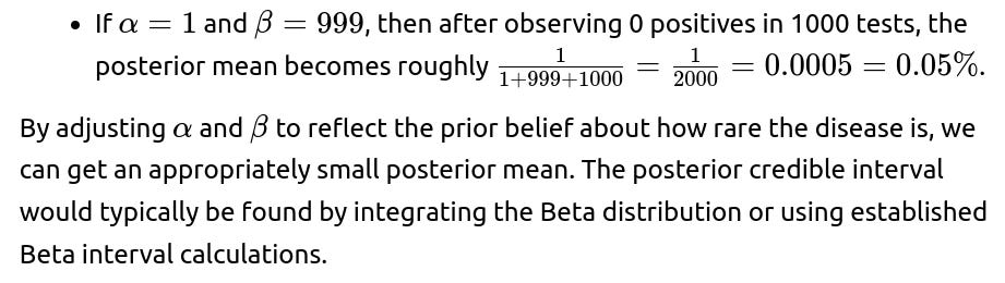
In this illustration, if we choose a uniform prior Beta(1,1), then after 0 positives in 1000 tests, we end up with Beta(1, 1001). The posterior mean is about 1/1002 ≈ 0.000997, or roughly 0.1%. The 95% credible interval will be from 0 to around 0.003, paralleling the frequentist confidence interval result.
This kind of code snippet demonstrates how you might practically estimate the probability in a Bayesian framework. If you believe the disease to be much rarer, you adjust the prior (alpha, beta) accordingly.
Likely final numeric answer
From a standard quick approach:
The frequentist rule of thumb says the disease probability in the city is most likely 0, but it is no bigger than about 0.003 (0.3%) with 95% confidence.
A Bayesian approach with a uniform prior would yield a posterior mean around 0.001 (0.1%), with a similar upper bound on the credible interval near 0.003. A more skeptical prior about disease prevalence (e.g., mean ~ 0.0001) might yield an even smaller posterior estimate.
Hence, the straightforward conclusion is that the probability is probably on the order of a fraction of a percent, with an upper bound that can be a few tenths of a percent depending on the specifics of the method used.
If the interviewer asks: “Why not just say the probability is zero since we saw zero cases?”
It’s true that the maximum likelihood estimate from the binomial model is 0. However, an estimate of exactly 0 is typically not realistic in practical epidemiological settings. There could be unobserved cases, sampling biases, or imperfect test sensitivities. Statistically, we also know we cannot prove the probability is exactly zero from finite data. Hence, we provide an interval or a posterior distribution that shows how small p can be while remaining consistent with zero observed positives in 1000 trials. The estimate is near zero, but not strictly zero.
If the interviewer asks: “How do you get that approximate bound of 3/n for zero positives?”

If the interviewer asks: “What if the test has a non-negligible false negative rate?”


From a frequentist perspective, one might solve for the p that makes this probability correspond to a certain confidence bound. In a Bayesian framework, we would re-compute the likelihood accordingly and update the prior on p.
The net effect is that any false negative rate means a higher possible prevalence for the same observation of zero positives. If your test misses 20% of actual cases, you cannot exclude the possibility that some fraction of those 1000 were in fact infected but tested negative.
If the interviewer asks: “Could the sample be biased or unrepresentative of the city?”
Yes. If the 1000 people tested are not representative—for instance, if they come from a demographic with different exposure or health outcomes than the general city population—then the result might not generalize. The assumption behind the binomial model is that each individual tested is an independent draw from the city population. In reality, you might have cluster effects or self-selection in testing. True random sampling is ideal but often not the practical reality in medical or epidemiological contexts. Hence, the overall city probability might differ if the tested group systematically under- or over-represents certain segments of the population.
If the interviewer asks: “Please detail how you’d communicate these results to non-technical stakeholders?”
In non-technical communication, it’s often enough to say:
“We tested 1000 people. No one tested positive. While we can’t say the disease is truly 0% in the city, our statistical estimate is that it’s probably well below 1%. A common rule of thumb puts an upper bound around 0.3%.”
We’d emphasize: “This result is consistent with a very low prevalence. However, it does not rule out that some cases exist—especially if the test can miss some cases or if the sample was not fully representative.”
We avoid stating “there is no disease at all,” because that can be misleading. Instead, we highlight that the data strongly suggests a small upper limit, subject to various assumptions.
If the interviewer asks: “How does the Bayesian posterior interval differ from a frequentist confidence interval?”
A frequentist confidence interval is an interval that would contain the true parameter in repeated sampling 95% of the time. It is strictly a statement about a procedure’s long-run behavior on hypothetical repeated experiments.
A Bayesian credible interval is a direct probability statement about the parameter itself given the observed data. It answers: “Given our prior and the data, there is a 95% probability that p lies in this range.”
In practice, for a large sample size or for relatively simple problems, the intervals can look numerically similar. But philosophically and interpretationally, they differ. For this scenario (0 successes in 1000 trials), both intervals will often cluster near zero with an upper bound around 0.002-0.003. The exact number depends on the chosen Bayesian prior or the frequentist confidence procedure.
If the interviewer asks: “Summarize the final numeric estimate and interpretation again?”
We usually quote:
MLE: 0%.
95% confidence (or credible) upper bound: roughly 0.3%.
Bayesian posterior mean (assuming a uniform prior): about 0.1%.
Bayesian posterior interval: from near 00 up to about 0.3%.
Hence, it is likely that the disease rate is very small, definitely under 1%, probably under 0.3%. The exact numeric estimate within that range depends on the assumptions (prior, test accuracy, sample representativeness).
If the interviewer asks: “What does this show about the difference between statistical significance and practical significance?”
It highlights how an event can be extremely unlikely (like seeing zero positives if the city had a 1% prevalence, you’d expect about 10 positives out of 1000). Observing zero is quite strong evidence that the prevalence is significantly less than 1%. From a practical standpoint, it means the disease is rare enough that targeted testing or certain interventions may be more cost-effective than broad-based city-wide measures. However, for diseases with serious outcomes, even a tiny prevalence can still be important. You would not want to say “ignore it altogether” if the disease is fatal or highly contagious.
If the interviewer asks: “How would you handle the case where the nationwide prior is extremely low, like 0.0001?”

If the interviewer asks: “Could you show me a minimal Python code snippet for constructing a confidence interval for the binomial proportion with 0 successes?”
Yes. One could use statsmodels or other libraries. A minimal example:
import math

n = 1000
x = 0
alpha = 0.05  # For a 95% confidence interval
# Use a basic approximate formula for the upper bound:
# 1 - alpha -> about 3/n if x=0 for large n
upper_bound_approx = 3 / n
print("Approximate 95% upper bound (rule of thumb):", upper_bound_approx)

# For an exact Clopper-Pearson interval, we could do:
from statsmodels.stats.proportion import proportion_confint
ci_low, ci_high = proportion_confint(x, n, alpha=alpha, method='beta')
print("Exact Clopper-Pearson CI:", (ci_low, ci_high))
If you run this, you’ll see ci_low is 0, and ci_high is around 0.00299 (0.299%), which aligns with the rule of thumb.
If the interviewer asks: “Give a final one-liner answer to the original question.”
If forced to give a single value, one might say: “It’s very likely below 0.3%.” Or one might say: “Based on the data, an upper 95% bound is around 0.3% for the prevalence in that city.” If using a Bayesian approach with a uniform prior, the posterior mean is around 0.1%. Either way, the estimate is extremely small.
Below are additional follow-up questions
What if the test is assumed to be perfect, but the population is extremely heterogeneous?
When the test itself is near 100% sensitivity and specificity, the main source of uncertainty shifts from test accuracy to the underlying variability in disease prevalence across subgroups of the population. In such heterogeneous settings, the overall city-wide probability of the disease isn’t necessarily uniform. One subgroup might have a higher prevalence, while most of the city has an extremely low prevalence. If we happened to sample 1000 individuals mostly from the low-prevalence subgroup, the test results could misleadingly indicate near-zero prevalence.
In statistical terms, the simple binomial model assumes each person’s probability p of having the disease is the same. That assumption breaks down if there are clusters of different p values. The typical approach would be to stratify the population by known risk factors or subpopulation identifiers (e.g., age groups, neighborhoods, occupations) and sample proportionally or oversample from higher-risk strata. Then we estimate prevalence within each subgroup and combine them (weighted by their proportion in the population) for an overall estimate.
A potential pitfall is ignoring the heterogeneity and concluding that the disease is almost nonexistent city-wide, even though pockets of higher prevalence might exist. This can happen if the sample missed or underrepresented those high-prevalence areas.
A real-world example could be if the disease is heavily localized among certain neighborhoods or communities. A random sample that fails to capture those communities accurately might yield a misleadingly low estimate. Hence, even with a perfect test, heterogeneity in the population requires careful sampling design or a stratified model. If unmodeled, it can lead to biased estimates of overall prevalence.
How does the sample size impact the ability to detect very low prevalence?
The sample size directly influences the power to detect low prevalence. Power, in this context, is the probability that a test of hypothesis (e.g., p>0) will reject a null hypothesis if a true nonzero prevalence exists. Suppose the true prevalence is extremely small, such as 0.1%. In a sample of 1000, the expected number of positives would be only 1. If we see zero positives, it might be statistically plausible that 0.1% is the actual prevalence (since on average 1 positive is expected, but 0 is not too unlikely). If we want a higher chance of observing at least one positive at that prevalence, we need a larger sample.
Increasing the sample size helps in two ways:
More expected positives. If p is small but nonzero, a larger n yields a higher expected count of positives, which helps confirm whether the disease is truly absent or merely rare.
Narrower intervals. Confidence or credible intervals shrink with more data, giving more precise estimates. With a bigger n, the difference between “true prevalence is zero” and “true prevalence is a tiny fraction” becomes easier to detect.
The main pitfall here is underestimating how large a sample is needed to detect extremely rare events. If the disease is on the order of 0.01%, even 1000 samples might not be enough to confidently observe a case. That might lead to an incorrect inference of near-zero prevalence, even though a small nonzero prevalence exists.
How would we incorporate strong prior evidence that this city differs significantly from national trends?
If the city is known for special conditions—such as a different climate, unusual demographics, or a very different health system—we may want to override or adjust the national prior. Instead of using a prior that the city’s prevalence matches the nationwide rate, we might set a prior that’s either heavier (if there are risk factors) or lighter (if there are protective factors).
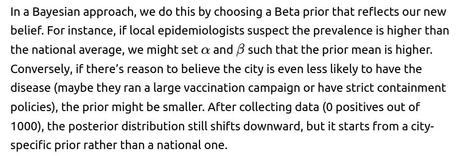
The challenge is determining how strong that prior evidence should be. If the prior is too strongly weighted (e.g., extremely high or low), it can overwhelm the data. If it’s too weak or uninformative, then we might ignore relevant city-specific knowledge. Balancing prior beliefs with observed data is the core of Bayesian inference, and it depends on domain expertise. The pitfall is ignoring real local factors or, conversely, using an unrealistic prior that can’t be justified by actual knowledge.
How would a real-time monitoring or longitudinal system for disease prevalence differ from a single cross-sectional sample?
A single cross-sectional sample captures a snapshot in time. If we want to track changes in disease prevalence across weeks or months, we might do repeated sampling or rely on continual test data from healthcare systems. A real-time or longitudinal monitoring approach might use:

In each new time step, we incorporate new observations (like “1000 more tested, 1 positive found”) and revise our estimate. This is more informative than a one-time estimate because it captures trends. The main pitfall is that if the disease prevalence starts extremely low but then spikes quickly, a system that updates too slowly (or uses outdated data) might not catch the surge in time. Another subtlety is ensuring that each new sample is representative over time, which is not always trivial. Also, if we rely on self-reporting or hospital data alone, selection bias can accumulate over time.
What if we want to combine data sources, e.g., official health records plus our random sample?
In practice, the best estimates may come from blending multiple data sources. We might have:
Official health records: Hospitals or clinics might record confirmed cases, but those records can be biased toward symptomatic or severe cases.
Randomly sampled survey: A smaller but systematically collected set of tests from the general population.
A Bayesian hierarchical model could incorporate these sources. The hospital data might inform an estimate of symptomatic or severe-case prevalence, while the random sample might inform overall prevalence (including asymptomatic cases). We might create a latent variable for the “true” prevalence and then have different likelihood models for each data source, factoring in each source’s biases or detection rates.
One major pitfall is double-counting the same individuals (overlapping data) or incorrectly assuming independence across sources. Another subtlety is reconciling different timescales or definitions of “case.” Official data might count “test positives,” while a random sample might detect “current infection.” If the definitions or timescales don’t align, we risk combining apples and oranges. The advantage is that multiple data sources often reduce uncertainty and yield a more robust estimate if carefully modeled together.
How do we handle a scenario where there might be localized hotspots or super-spreader events but still zero observed positives in our random sample?
If there are potential hotspots—say, one specific cluster, like a nursing home or a large indoor gathering—a purely random sample from the entire city might miss that cluster if it’s small relative to the city population. That can give a false sense of security. The disease might still be present but contained in that hotspot.
To handle this, epidemiologists sometimes use:
Cluster sampling or oversampling: If they suspect certain hotspots, they specifically test those areas more thoroughly.
Spatial or network-based models: Instead of a single city-wide prevalence, they model prevalence as a function of location or social networks.
Seeing zero positives in a city-wide random sample does not guarantee zero hotspots; it could simply mean that the hotspot is small and was missed. The pitfall is concluding no risk city-wide. In reality, an outbreak could be brewing in a corner of the city. Hence, we might combine random sampling with targeted hotspot surveillance. If both show zero positives, that’s more convincing.
What if we only tested 100 or 200 people, not 1000?
The smaller the sample, the wider the confidence or credible interval. Observing zero positives in 200 tests is less informative than zero positives in 1000 tests. For instance:

How do we handle diseases with significant latent periods where the test might not detect early infections?
Some diseases have an incubation or latent period during which tests (especially certain types of tests, like antibody tests) might not detect the infection. For example, if it takes two weeks from infection before a person tests positive, someone recently infected would appear negative even though they are infected.
We can incorporate a time dimension in the test sensitivity model. Instead of a single sensitivity value, we have a sensitivity function that depends on how long since exposure. If the tested individuals were in early stages of infection, the probability of detection is lower. Hence, the probability of seeing zero positives might be higher than you’d assume under a single-sensitivity assumption.
A real-world pitfall is ignoring these dynamics. If we tested 1000 people during a time window that coincides with the latency period, many infections could go undetected. We might incorrectly conclude near-zero prevalence. One approach is repeated testing or using a test that detects earlier stages (like PCR for viral RNA) rather than relying on an antibody test that only becomes positive after a longer period.
Could we apply a non-parametric or bootstrapping approach to estimating prevalence instead of a binomial model?
Yes, non-parametric or resampling techniques can be used, but they typically still rely on the assumption that each sample is an i.i.d. draw from the city population. For instance, one might do a bootstrap by repeatedly sampling from the observed test results, but if we have only zeros, the bootstrap distribution also yields zeros.
In effect, bootstrapping with zero positives in the data will often produce an estimated distribution heavily centered at zero, unless some smoothing or prior is introduced. In many epidemiological scenarios, the parametric binomial model is straightforward and well-accepted. A purely non-parametric approach might not provide much additional insight when you observe all negatives.
One pitfall is that a naive bootstrap could yield no new information if your empirical data has no positives. Another subtlety is that bootstrapping doesn’t incorporate an informative prior that the disease is just rare. So in practice, a parametric or Bayesian approach is often more interpretable. Still, if you had a set of positive results from a bigger region, you might do partial pooling or advanced resampling. But with zero positives, the parametric binomial or a Beta-Binomial approach typically suffices.
What if the disease presence in the city is correlated across families or neighborhoods (not independent Bernoulli trials)?
When infection status is correlated—say, within families or neighborhoods—the assumption of independent Bernoulli trials doesn’t hold. This can cause underestimation or overestimation of the variance in the number of cases. Typically, binomial confidence intervals assume independence. But if entire households tend to share exposure, either you see “clusters” of positive or negative results.
If your sample includes families or neighborhoods, the real effective sample size might be smaller than it appears, because each household’s results are correlated. This leads to narrower or incorrectly calculated intervals if you ignore that correlation. One approach is to move to a Beta-Binomial or hierarchical model that can capture within-group correlation. Another approach is carefully sampling one individual per household, ensuring independence.
The pitfall is ignoring the correlation and using standard binomial methods, which leads to overly optimistic confidence intervals. In other words, you might claim more certainty about your estimate than is actually warranted, because each test is not truly independent evidence.
What if the city health department or stakeholders want a guaranteed upper bound at higher confidence (e.g., 99.9% instead of 95%)?
Raising the confidence level from 95% to 99.9% widens the interval, meaning the upper bound on prevalence increases. For instance, using the rule of thumb or exact binomial intervals at 99.9% confidence might push the upper bound well above the 0.3% figure we get at 95% confidence.

What if there’s a risk of test contamination or a small but nonzero risk of false positives?
Even if no positives appeared, we might wonder if the test could produce false positives or if the lab might mix up a sample. Usually, that would result in a few positives, not zero. So ironically, false positives wouldn’t lower our estimate further, they’d raise it or at least create some noise. However, the presence of potential contamination can cast doubt on any result. If the lab might discard suspicious results or retest suspicious positives more than negatives, that could bias the results in favor of fewer positives reported.
Another subtle scenario is if a lab systematically discards borderline positive tests to “be sure” or if they assume the disease is rare and attribute borderline results to errors. This sort of confirmation bias can artificially drive positives to zero. The pitfall is that all the classical binomial or Bayesian formulas assume accurate classification of disease status. If we suspect systematic lab or test biases, the entire inference process must be revisited with a realistic measurement-error model.
How can we extend this analysis to account for mortality and recovery rates?
If we’re considering a disease that has a certain mortality rate or a known recovery period, then prevalence at a specific point in time is a function of new infections, recoveries, and deaths. Over a longer window, we may need a compartmental model (like SIR or SEIR in epidemiology):
S = Susceptible
E = Exposed (latent)
I = Infectious
R = Recovered (or removed)
Prevalence is essentially the proportion of the population in the “I” state (or possibly “E” + “I” if the test detects early infection). If we test 1000 people at a random time, 0 positives might mean the “I” compartment is very small or practically zero. But if transitions in and out of “I” happen quickly, we might be testing at a moment of low incidence. Another time, the city might experience a surge.
The pitfall is using a simple cross-sectional estimate from a single time point to project or forecast the disease course without considering dynamic factors. The more accurate approach is to incorporate the zero-case observation as an initial condition or constraint in a dynamic model. Then we can project forward or backward, factoring in infection rates, mortality, and recovery. This is complex but more realistic in certain epidemiological contexts.
How might we adapt the approach if the question was about “probability of a rare event” more generally, not just disease prevalence?
The logic extends to any scenario where we’re trying to estimate a low probability of occurrence—like product defect rates, financial default rates, or event occurrences in a system. Whenever we observe zero occurrences in a sample, the same binomial-based intervals or Bayesian updates apply. For a Poisson process with a low event rate, we can also use a Poisson assumption in place of binomial. If we sample 1000 days (or 1000 units) with zero events, we get an estimate or confidence interval for the underlying rate.
A potential pitfall is mismatch between real-world processes and the chosen model. For instance, if events cluster in time, a Poisson or binomial assumption might be wrong. The takeaway is that the math is similar, but we must ensure the underlying assumptions—independence, distribution type, sample representativeness—hold for the general scenario.
How do we reconcile multiple intervals or estimates that come from different methods (frequentist vs. Bayesian, or from different data subsets) that appear contradictory?
Contradictory intervals might arise if, for instance, a frequentist approach on one data subset yields an upper bound of 0.4%, while a Bayesian approach with a strong prior on another subset yields 0.1%. This can happen if the subsets differ, or if the prior in the Bayesian method strongly pulls the estimate down.
We reconcile them by asking:
Are the datasets truly comparable? Maybe one subset was tested at a different time or in a different population segment.
How strong is the Bayesian prior, and does it properly reflect reality? If the prior is too optimistic or extremely tight, it might artificially reduce the posterior.
What is the confidence level or credible interval used in each approach? A 99% frequentist interval vs. a 90% Bayesian credible interval might yield ranges that don’t overlap simply because of different confidence levels.
A combined or hierarchical approach might help unify the sources. The main pitfall is assuming that each “interval” must match exactly. Different methods can yield different intervals, especially with small counts and strong priors. Investigating the assumptions behind each method is essential for a coherent final conclusion.
How would we modify the approach if we suspect under-reporting of negative test results, or incomplete data?
Sometimes data might only be recorded for positive tests, or negative results are less diligently recorded. That would effectively sample more from positives, skewing the sample. In a scenario where we have 1000 negative tests recorded, but an unknown number might not have been reported, our sample is incomplete. We can’t treat it as a random sample of the city.
One approach is to attempt to estimate the missing data fraction. If we know that only half of negative tests are typically reported, we can partially correct for that under-reporting. But that correction requires additional assumptions about how negatives are missed. In a Bayesian framework, we can place a prior on the fraction of missing data and incorporate that into the likelihood. The pitfall is that any error in that missing fraction assumption drastically changes the prevalence estimate. Without reliable data on the extent of under-reporting, the uncertainty grows considerably.
How do we handle follow-up studies if we eventually find a small number of positives?

In a frequentist approach, we can pool the data: total tests = 1500, total positives = 1. Then we do a binomial estimate with n=1500, x=1. Or we can do separate interval calculations for each wave of data and combine them via meta-analysis or a weighted approach. The pitfall is ignoring the time gap or changes in conditions between the two sampling periods. If the disease prevalence changed in the intervening period, pooling might not reflect a single consistent probability. One might need a time-varying model to properly handle that shift in prevalence.
How might budget and logistical constraints influence the approach or interpretation of results?
In the real world, testing 1000 people can be expensive. Decision-makers might only want to test 200 people. But as discussed, a smaller sample means wider uncertainty. Another scenario is that tests are costly, but we can do them in multiple small waves over time. This sometimes yields more information if the disease prevalence changes or if we want to quickly detect an outbreak.
Budgetary constraints can also influence the design of a testing program. We might do adaptive testing: start with a smaller sample, see if positives appear, and expand if evidence suggests non-negligible prevalence. The pitfall is concluding that zero positives from a small sample is enough to claim near-zero disease. For extremely rare diseases, a large enough sample or a repeated-sampling strategy is crucial to reduce the chance that we’re simply missing the few positive cases.
If herd immunity or vaccination coverage is very high in the city, how does that alter the interpretation of zero positives?
High vaccination coverage or partial immunity might lower the effective disease prevalence. Observing zero positives can be consistent with a high level of protection in the population. However, “prevalence” in that context might be different from the “probability of the disease in an unvaccinated individual.” If most people are immune, the overall prevalence is small, but the risk for the unvaccinated could still be higher than the city-wide average.
In practical epidemiology, we might measure the “breakthrough infection” rate among vaccinated individuals separately from the “infection rate” among unvaccinated. If we don’t distinguish, the zero positives might be mostly among vaccinated individuals. If the unvaccinated population is small, we might not have tested enough unvaccinated individuals to see a positive. The pitfall is concluding “nobody is infected,” but not realizing that among the handful of unvaccinated folks, prevalence might still be meaningful if the disease thrives there. This underscores the importance of understanding the composition of the tested group and the overall immunity landscape.
How do we refine our model if the disease is highly seasonal or has known fluctuation patterns?
Seasonal diseases (e.g., influenza-like illnesses) might have low prevalence in the off-season and higher prevalence in peak season. Observing zero positives in the off-season is not surprising. To estimate prevalence, we may need a seasonal model capturing p(t) as a function of time of year. If the sample was taken in the disease’s typical “low season,” it might not reflect the potential prevalence that could occur in the “high season.”
Statistically, we could use a sinusoidal or piecewise function for the prevalence over time, or a state-space model with seasonal components. The pitfall is ignoring the time of measurement. A naive approach concluding near-zero disease year-round from a test done at the low point can be very misleading. Epidemiologists often do repeated surveys across the year or over multiple years to handle seasonality. For a single snapshot, they usually interpret zero positives in context: “We tested in the off-season, so that’s consistent with near-zero at this moment, but not necessarily a forecast for the peak season.”
Could a hierarchical Bayesian approach be used to borrow strength from data on other diseases in the same city or from the same disease in neighboring cities?
Yes. Hierarchical modeling can allow partial pooling across multiple diseases or across multiple cities. For example, if City A, B, and C are geographically similar, we might treat the disease prevalence in each as drawn from a common hyper-distribution. Observing zero positives in City A but some positives in City B might shift A’s posterior a bit upward because it’s plausible they share risk factors. Or if we see no positives in all three, that jointly increases confidence that the region has very low prevalence.
A big pitfall, though, is incorrectly assuming cities or diseases are sufficiently similar. If one city has unique features (like high vaccination rates or strong travel restrictions), pooling data with other cities might artificially inflate or deflate estimates. Proper hierarchical modeling requires verifying that the grouping factor (cities, diseases) is indeed coherent. Otherwise, you get erroneous “borrowing” that misrepresents local realities.
If the local government uses zero-positives to cut back on testing, what are the risks?
This is a policy pitfall. After seeing zero positives in a sample of 1000, officials might reduce testing programs to save costs, believing the disease is virtually absent. That could be risky if:
The disease is still present but at a very low level. Reduced testing might miss the early signals of an outbreak.
New variant or new wave. Conditions can change; external introductions of the pathogen might cause a sudden increase.
Sampling was unrepresentative. If the initial sample was incomplete or biased, the city might incorrectly think there’s no problem.
An ongoing surveillance approach is often recommended, even if scaled down, to promptly detect changes in prevalence. Another strategy is sentinel surveillance: testing selected clinics, high-risk groups, or random samples at regular intervals. The main pitfall is that zero positives is not an absolute guarantee of no disease; it’s just strong evidence that the prevalence is very low at that moment.
How does the ratio of infected to total population differ from incidence, and does that matter here?
Prevalence typically refers to the proportion of the population that is currently infected (or has a disease) at a given time. Incidence refers to the rate of new infections per unit time. The question we addressed focuses on prevalence: “What is the probability that someone has the disease now?”
However, if the disease is acute and short-lived, the prevalence might be very low, even though the incidence (new cases per day) might be more substantial for short intervals. For instance, a disease that lasts only a few days might never accumulate large prevalence. If the question was about incidence, we would need data on how many people newly become infected over time, which is different from “how many are infected at a single time.”
The pitfall is conflating the two measures. A city might have zero currently infected individuals at a certain moment (prevalence near zero), but that doesn’t mean they have a zero rate of new infections if, for example, the disease has short duration but recurs in waves. Clarifying whether the question is about point-prevalence or incidence is crucial for correct interpretation.
If results indicated zero infected individuals, how might community testing strategy shift toward sampling more at-risk subgroups?
When zero positives come from a broad random sample, the next step might be more targeted testing. We’d direct resources where the disease is most likely to appear, such as travelers arriving from high-prevalence regions or individuals with known risk factors.
The idea is two-tiered:
General screening: We do a broad random sample to gauge baseline prevalence.
Targeted follow-up: If we see zero in the broad sample, but we still have concerns about specific high-risk subgroups, we do a separate or additional test in those subgroups.
The pitfall is to assume that one broad sample that yields zero positives means we can ignore high-risk subgroups. Conversely, focusing too heavily on high-risk groups might skew city-wide prevalence estimates if we want to continue measuring the overall level. Balancing general population testing with risk-focused testing is often the best approach, especially when resources are limited.
Could we incorporate knowledge about disease transmission dynamics (like R0) into the prevalence estimate?
R0 (the basic reproduction number) or the effective reproduction number Re can inform how quickly a disease would spread if introduced. If a disease has a high R0 but we still see zero positives, it might mean we’re in a lucky scenario where no introduction events have occurred yet, or the population has immunity. This knowledge might shape a Bayesian prior, indicating that if the disease were present, it would likely have spread to produce some positives. Observing zero might be stronger evidence for extremely low prevalence than if it’s a disease with low R0.
However, direct integration of R0 into a simple binomial or Beta-Binomial analysis is not typical unless we build a dynamic transmission model. The pitfall is mixing up theoretical transmission potential with actual observed data. R0 alone can’t measure current prevalence—some highly transmissible diseases might still be absent in a particular location if they haven’t been introduced or if controls are in place. Combining these methods in a full epidemiological model can be powerful but is significantly more complex than the static binomial approach.
What if the disease has known subclinical or asymptomatic cases that even a perfect test cannot detect unless they’re in a specific phase?
Some diseases manifest in waves of detectable biomarkers. If the test only detects the pathogen during symptomatic or a particular phase, asymptomatic carriers might test negative. This is effectively a test sensitivity issue, but with the added complexity that the sensitivity depends on symptom phase.
We might extend the model to:
Identify the fraction of cases that remain asymptomatic or subclinical.
Estimate the fraction of those asymptomatic cases that still test positive (some tests can detect the pathogen even when asymptomatic).
Combine these factors in the likelihood function for observing zero positives.
If the fraction of subclinical carriers is high and the detection rate in that phase is low, it’s plausible to see zero positives even if the true prevalence is not zero. The pitfall is using a single sensitivity figure that only applies to symptomatic individuals and ignoring subclinical or asymptomatic states. This leads to underestimation of the true prevalence if we rely purely on test outcomes.
How do we handle logistical constraints such as batch testing (pool testing) where multiple samples are combined to reduce costs?
Pool testing involves mixing, say, 10 samples together and running one test on the pooled sample. If negative, we conclude all 10 are negative. If positive, we individually retest. It’s a common approach to reduce costs when prevalence is expected to be very low.
If all pooled tests come back negative, we effectively have zero positives across many individuals, but we must consider the possibility that a single infected sample in a pool might go undetected if the viral load is diluted below the test’s detection threshold. That modifies the probability model. The risk is higher false negatives in pooled samples, especially if the pool size is large, or if the test’s detection threshold is borderline.
Hence, to estimate the overall city prevalence, we must adjust the binomial or Beta-Binomial model to account for pooling efficiency and any test sensitivity changes due to dilution. The pitfall is applying the standard binomial formula to pooled results, ignoring the possibility that a small number of positives could be missed. If we don’t correct for that, we might be overly confident in concluding zero or near-zero prevalence.
What if local clinicians suspect mild cases are going unreported due to a cultural tendency to avoid medical testing?
Cultural or behavioral factors can lead to self-selection: people who feel ill may avoid testing to keep working or to avoid stigma. This introduces a hidden segment of untested but possibly infected individuals. The 1000 tested might be the more health-conscious population that believes they’re not infected or is comfortable reporting to clinics.
Statistically, this means the tested sample might not be random—it’s a self-selected subset with possibly lower prevalence. The real city-wide prevalence could be higher. A solution is to do an actively recruited random sample (like going door-to-door or offering incentives). If that’s not feasible, we might attempt a selection-bias correction model. The pitfall is ignoring these cultural factors, leading to an underestimate. If mild symptomatic individuals systematically avoid testing, we might incorrectly conclude zero prevalence from an unrepresentative sample.
How might contact tracing results or known contact networks inform the prevalence estimate?
Contact tracing data can reveal how many close contacts a confirmed positive had, how many tested negative or positive, etc. This can be integrated into a more elaborate network model of disease spread. If contact tracers find no evidence of spread within the city (no new positives among hundreds of close contacts), that suggests a very low prevalence or that the disease was never introduced to begin with.
A Bayesian network model might incorporate each contact event as an edge in a graph, with a probability of transmission if one node is infected. Zero positives among traced contacts is strong evidence of minimal or no presence in the city. The pitfall is that contact tracing is rarely 100% complete: some contacts may be missed, or some might refuse testing. Also, a zero-case scenario might discourage thorough contact tracing, so we have limited data. If there was an index case who left the city or was never tested, we might have missed an introduction event. Combining random testing with contact tracing can yield a more holistic picture, but it’s methodologically complex to unify those data sources in a single estimate.
What if, after seeing zero positives, we do a second test on exactly the same 1000 individuals? Does that improve our estimate?
Testing the same group twice can provide some additional information, particularly about test reliability or disease incidence over a short period. If, for example, the disease has an incubation period or if the second test is a different type with different sensitivity, combining the results might reduce the chance we missed someone who was infected. However, if we do a back-to-back test on the exact same individuals at roughly the same time, the second test might be almost redundant if the disease status wouldn’t have changed.
In a standard binomial framework, if the prevalence is stable and we get all negatives twice from the same group, it doesn’t drastically change the conclusion that the prevalence is very low for that group. The pitfall is to double-count the results as if they were two independent samples from the city. They’re not entirely independent if it’s the same people. On the other hand, if we space out the tests by a few weeks, it might provide more robust information about new infections. But if the question is just “What is the city prevalence at a single point in time?,” retesting the exact same individuals soon after yields diminishing returns.
What if we want a decision rule, like “we declare the city disease-free if the posterior probability that p>0.001 is less than 5%?”

This approach is more direct than constructing a credible interval. We have a decision boundary at 0.1%. The pitfall is that the chosen threshold might be arbitrary. Why 0.1%? Or 5% probability? The choice might be driven by policy or risk tolerance. Also, if the prior is overly optimistic or pessimistic, we might too quickly or too slowly meet that decision threshold. The advantage is clarity: the final statement is a direct measure of “We are X% certain that the prevalence is below Y%.”
How could we incorporate the notion that the disease might have an extinction probability if it falls below a certain prevalence?
Some epidemiological models posit that if an infectious disease falls below a critical fraction, it may die out entirely (basic branching process logic). Zero positives might signal that the disease failed to sustain transmission. If we adopt a branching process model, we might estimate the probability that the disease has “gone extinct” in the city. Observing 0 cases in a large sample can increase the posterior probability that the chain of transmission ended.
However, we must be cautious: local extinction is possible, but reinfection from outside sources is also possible, so “extinction” might be temporary. The pitfall is proclaiming the disease extinct city-wide when it might still exist in an untested cluster or be reintroduced from outside. Nonetheless, for diseases known to have a critical community size or threshold, the observation of zero positives in 1000 samples is strong evidence that the chain of transmission is currently not self-sustaining. This again requires a dynamic model that extends beyond a static binomial approach.
Could advanced machine learning techniques, such as Bayesian neural networks or Gaussian processes, help in this estimation?
In principle, yes. For example, if the city is large and we want a spatially varying prevalence model, a Gaussian process can be used to model the prevalence function across geographical coordinates. If we have zero positives from certain sampled locations, that suggests a near-zero mean function in those areas. Additional data from different neighborhoods might feed into the GP to refine the city-wide map. Or a Bayesian neural network might incorporate covariates (e.g., population density, mobility patterns) to estimate prevalence.
However, if the number of positives is zero or extremely small, these advanced models can suffer from data scarcity. They might overfit or fail to converge on meaningful parameters. The advantage is they can incorporate complex dependencies and side information. The pitfall is that for something as simple as “0 out of 1000 tested,” classical methods (binomial or Beta-Binomial) might be more straightforward and robust, especially if we lack extensive features to feed into ML models. In real-world scenarios, advanced ML might be helpful if we have rich data about each individual or region. But for a quick, straightforward prevalence estimate with zero positives, the classical approach is often sufficient and more interpretable.
What if public perception demands a definitive statement (“the disease is nonexistent”) but from a scientific standpoint we can only say “it’s below X%”?
This is a classic science communication challenge. Statistics can’t prove a negative absolutely; we only provide intervals or probabilities. A demand for a definitive zero is impossible to meet. The best we can say is: “Based on our sample, we’re highly confident the prevalence is below some small threshold.”
The pitfall is that authorities or the media might spin zero positives as total absence. Then, if a single case appears later, it could damage trust in the data or the health department. The recommended approach is to carefully phrase the conclusion, emphasizing that zero positives in 1000 tests strongly suggests a very low prevalence, but not a literal zero. Using intervals (e.g., “very likely below 0.3%”) or probabilities (e.g., “95% chance it’s below 0.3%”) manages expectations better. Scientific caution is key, even though it may not align perfectly with public desire for certainty.
What if the city’s population is quite large (e.g., millions) and 1000 tests is a relatively small fraction, but we still see zero positives?

What if the city suspects the disease is so rare that they only tested the highest-risk people (like symptomatic individuals), and still got zero positives?
Testing only high-risk or symptomatic individuals and finding zero positives is very strong evidence that the disease is absent in that specific group. If the disease typically manifests with clear symptoms, that lowers the chance that it exists silently among symptomatic people. But it says less about truly asymptomatic or mild cases in the broader population.
In a binomial framework, we are no longer sampling from the general population with a probability p. Instead, we’re sampling from a subpopulation with presumably higher disease probability. Observing zero there might push us to an even lower estimate of city-wide prevalence, or at least for the prevalence among symptomatic individuals. The pitfall is confusing the result among symptomatic or high-risk individuals with the overall city prevalence. The city might still have infected individuals who do not present strong symptoms or do not consider themselves “high-risk.”
How might privacy laws or data regulations (e.g., HIPAA) limit the precision or sample design we can use?
Privacy concerns might prevent us from collecting granular data on each test subject’s demographics, location, or risk factors. Consequently, we can’t stratify or properly model subpopulation prevalence. We might only have aggregate data like “0 positives out of 1000.” This hamper’s more sophisticated Bayesian or hierarchical approaches that rely on covariates.
Moreover, we might be unable to recontact individuals for follow-up tests or link test results to hospital records. That can reduce the reliability of our estimates. The pitfall is that if our sampling is forced to remain anonymous or aggregated, we lose the ability to check for repeated tests, analyze group-based differences, or correct for confounders. We have to rely on simpler, coarser statistical approaches, which might widen intervals or require stronger assumptions about representativeness.
Could we design an adaptive sampling strategy that adjusts how many additional people to test based on the observed negatives so far?
Yes, an adaptive or sequential sampling design is common in industrial quality control or medical surveillance. The idea:
Start by testing a small group (e.g., 200 people).
If we see zero positives, check the posterior or confidence interval. If the upper bound is above a certain threshold, we test more individuals to narrow it.
Continue until the upper bound on prevalence is below a target threshold (e.g., 0.2%) with high confidence.
This approach can save resources if disease truly is very rare, but it can also quickly scale up if early results suggest a non-trivial prevalence. The pitfall is not setting clear stopping criteria. If we keep testing indefinitely to push the upper bound lower and lower, we might run out of resources. Also, each additional round of testing must be random or representative to ensure valid inferences, which can be logistically complex.
If the city is planning an event (e.g., a large festival), how does zero positives in a sample inform risk assessment for that event?
Zero positives is reassuring, but risk assessment for an event depends on:
Time-lag: The tests reflect the situation at sampling time, not necessarily the future event date.
Potential introduction from outside: People from elsewhere may come to the festival, so local zero prevalence doesn’t guarantee no one will bring in the disease.
Population mixing at the event: Even if local prevalence is near zero, a single infected visitor could spark an outbreak if transmission at large gatherings is efficient.
Hence, from a public health standpoint, we might combine these zero-positive results with:
Travel data: Are people coming from regions with higher prevalence?
Vaccination or immunity checks: Are attendees required to show negative tests or proof of vaccination?
Mitigation measures: Mask requirements, social distancing, or capacity limits.
A pitfall is overconfidence in the city’s data while ignoring external sources of infection. Another subtlety is that a large event might change contact patterns drastically, so a near-zero city prevalence might not remain near zero if a single infected attendee arrives. Thus, zero positives is good news, but event-level risk must consider multiple factors beyond the local snapshot.
How does the uncertainty around each test’s specificity matter if we found zero positives?
Specificity is the true negative rate. If a test is less than 100% specific, it means some negative results might actually be false negatives—but typically specificity relates to false positives (so, a test with less than 100% specificity might incorrectly label healthy people as positive). Because we got zero positives, specificity doesn’t come into play directly for a negative classification. However, one subtlety is:
If the test had less than perfect specificity, it might produce some false positives in a large sample. Yet we got zero positives. That suggests either an extremely small prevalence or the specificity might be better than we thought.

Could partial data on positivity from older tests or adjacent time frames be combined with the current zero-positives to refine the estimate?
Absolutely. If we have historical data—for instance, last month 2000 people were tested, and 2 positives were found, then this month 1000 were tested with 0 positives—that can be combined in either a frequentist or Bayesian approach. We can pool the data (3000 tested, 2 positives) to get a single prevalence estimate, or we can separate them by time period and do a time-series approach.
A Bayesian approach might treat each month’s data as a separate binomial trial with a prevalence that evolves slightly over time. The posterior from the first month becomes the prior for the second month, etc. The pitfall is ignoring the time dimension. If prevalence changes from month to month, simply pooling might be misleading. Also, if the sample is not comparable across months (different demographics or testing criteria), mixing them without adjustments is risky. But done carefully, older data can reduce overall uncertainty. The new zero positives strongly suggests a downward shift in prevalence compared to the older data with 2 positives, leading to an updated, smaller estimate for the current time frame.
If the city leaders want a margin of safety, how should they interpret these statistical intervals?
Leaders might adopt a conservative stance: even if the 95% upper bound is 0.3%, they might plan for the possibility that 0.3% is real. This is especially relevant if the disease is dangerous or has severe consequences. In practice, they might use the upper bound in worst-case scenario planning. For instance, if the city’s population is 1 million, 0.3% would mean up to 3,000 infected individuals. That’s not trivial if the disease is serious.
Thus, city leaders might implement proportionate measures even though the central estimate is near zero. The pitfall is ignoring the difference between the central best estimate and the upper bound. Overly conservative policy might be expensive or disruptive. At the same time, ignoring the upper bound might create complacency. A balanced approach is to weigh the worst-case scenario from the confidence interval against costs and other risk factors (like how quickly the disease might spread).
Could “zero positives in 1000” be used to approximate a p-value for testing the hypothesis p=0.01 or p=0.005?

This approach is a classical hypothesis test. The pitfall is that p-values can be misinterpreted as the probability the city’s prevalence is at least 0.01, which is not correct. It’s just the probability of seeing zero positives if the true p=0.01. Also, we can test various hypothesized values. This is less commonly done in epidemiological practice compared to interval estimation or Bayesian updating, but it can be used for quick check of a specific threshold.
If we suspect strong confounding variables (e.g., the sample is only young adults) how do we adjust the estimate to the entire city’s age distribution?
If the tested sample is primarily young adults, but the entire city has a range of ages, we need a post-stratification adjustment. If disease prevalence strongly depends on age, a direct inference from a mostly young sample to the entire city might be biased. One solution is to:
Estimate age-specific prevalence within the sample (though we have zero positives, so it’s challenging).
Weight those age-specific estimates according to the city’s known age distribution.
Because we have zero positives in each age bracket of the sample, we might do a Bayesian approach with a small prior for each bracket. Then a partial pooling or hierarchical approach can share information across age groups. The pitfall is small sample sizes in some brackets. If older adults are underrepresented, we have little direct evidence about that group. A carefully stratified sampling design from the start would have avoided the confounding. But if we must adjust after the fact, we rely on assumptions about how the disease prevalence differs by age. If those assumptions are off, the final city-wide estimate could still be biased.
How does the type of test (antibody vs. antigen vs. PCR) affect the interpretation of zero positives?
Antibody test: Typically measures whether an individual had the infection in the past. If the disease was never present or only recently introduced, an antibody test might not detect it yet. Zero positives might reflect either no prior infection or that not enough time has passed for antibodies to develop.
Antigen or PCR: Detects current infection. Zero positives means no current active infection among those tested at that moment. However, it says little about past infections if individuals have already cleared the virus.
Hence, we must be clear which aspect of infection we’re measuring. Observing zero antibody positives could mean the disease was truly absent historically, or that the population is newly exposed and hasn’t developed antibodies. Observing zero antigen/PCR positives means no active cases at the test time, not necessarily zero overall exposure. A pitfall is mixing these test types without clarity, leading to confusion about whether we’re measuring current or past infection rates.
What if the disease is so severe that infected individuals immediately seek treatment, so you’d never find them randomly in a street sample?
Certain diseases (like Ebola or other severe infections) may drive symptomatic individuals rapidly into hospitals, making them unlikely to be found in random community testing. Then a random sample that yields zero positives might simply be missing the cases that are already hospitalized. To accurately estimate prevalence, we might need to include hospital data or do a thorough check of recently hospitalized individuals.
A potential pitfall is concluding the disease is absent in the entire city just because no one on the streets tested positive. In reality, the cases might be quarantined or in specialized units. This again highlights the importance of knowing the natural history of the disease and how that affects the chance of encountering infected individuals in any sampling method.
Could we leverage experts’ opinions or existing epidemiological models to define a more informative prior rather than a generic Beta distribution?
Yes, one common approach is eliciting a prior from domain experts. For example, local epidemiologists might say, “We believe there’s an 80% chance the prevalence is between 0.05% and 0.2%, and almost no chance it’s above 1%.” We can translate that into parameters for a Beta distribution or even piecewise distributions. That prior can be combined with the binomial likelihood from the sample.
The advantage is more realism than a uniform or ad-hoc prior. The pitfall is subjectivity—experts could be wrong, or might have bias. If the data strongly contradicts the expert prior, we must rely on the posterior to reflect that tension. And if 0 positives appear, it might drastically reduce the plausibility of the expert’s higher estimates. This can cause friction if experts are hesitant to revise their beliefs. Proper use of Bayesian methods demands we let the data override prior beliefs when there’s a strong discrepancy.
If we repeated the test on 10,000 people and still got zero positives, does that definitively prove no disease is present?

Practically, 10,000 tests might make us very confident that the disease is not widespread. But a small outbreak or single-digit cases in a city of millions could still be missed. The pitfall is complacency. A surprise outbreak might still occur if conditions suddenly change or if a case enters from outside. It’s safer to say “the disease is extremely rare or possibly absent,” not that it’s definitively nonexistent.
Does zero positives imply anything about the risk of future outbreaks?
Not necessarily. Zero positives only shows that at the time of sampling, there were no current detected cases. If the disease is highly transmissible and arrives with a single infected traveler, an outbreak can occur quickly. If the local population isn’t immune, the risk of future outbreaks depends on external factors (travel, neighboring regions, wildlife reservoirs, etc.). Zero positives might reduce the probability that an outbreak is already silently spreading, but it doesn’t remove the risk of future introductions.
The pitfall is ignoring external introduction. Diseases don’t respect city boundaries. A city with zero positives can become a hotspot if an infected person arrives and conditions favor rapid transmission. Public health policy often focuses on surveillance at points of entry or ongoing random tests, even if the current prevalence is near zero, to catch new introductions early.
What if “0 out of 1000” is a simplified summary, but in reality, a small fraction of tests were inconclusive?
Inconclusive or invalid tests are common in practice. If some portion—say 50 out of 1000—were invalid and had to be discarded or repeated, we effectively only have 950 valid negatives. Or if inconclusive results are a separate category, we need to figure out how to incorporate them. Some inconclusive tests might have been positive but unreadable, or might simply be test-lab errors.
One approach is to treat inconclusives as missing data. If we re-run them or eventually classify them, we can finalize the count. If we can’t retest them, we might incorporate a modeling assumption that inconclusives have the same probability of positivity as the overall sample or possibly a different probability if we suspect they were borderline. The pitfall is incorrectly counting inconclusive results as negatives or ignoring them altogether, which might bias the prevalence estimate. A robust method either excludes them properly or accounts for them with a missing-data approach, potentially introducing more uncertainty.
How might we respond if a local news headline runs “Disease totally eradicated in City X!” citing zero positives?
As a statistician or data scientist, the correct response is to clarify that zero positives in 1000 tests strongly suggests a very low prevalence but does not prove eradication. We can provide the statistical intervals or Bayesian posterior distribution to show that there remains a small but nonzero probability that the disease exists in a tiny fraction of the population.
The pitfall is in public misunderstanding or sensationalism. The phrase “eradicated” implies the disease is gone with 100% certainty. We’d caution that while the evidence is good that the disease is rare or absent, ongoing surveillance is prudent. A single moment of zero positives doesn’t guarantee zero future risk. This is a classic communication challenge: bridging the gap between statistical nuance and news-friendly language.