
ML Interview Q Series: Bayesian Updating Predicts Show Hit Probability Using Rater Feedback

Browse all the Probability Interview Questions here.
18. Before a show is released, it is shown to several in-house raters. You assume two types of shows: hits (80% chance that any viewer likes it) and misses (20% chance). Prior: 60% hit, 40% miss. After 8 raters, 6 liked it. What is the new posterior probability that it is a hit?
Understanding Bayesian updating in this scenario requires carefully applying the likelihood of seeing the observed evidence (6 likes out of 8) given each hypothesis (show is a "hit" vs. show is a "miss"), combined with the prior probabilities (60% for hit, 40% for miss).
Bayesian Reasoning for This Problem
Bayesian inference suggests that we take our prior belief about whether a show is a hit or a miss, calculate the probability of observing the evidence (6 out of 8 raters like it) under each hypothesis, and update our belief to get the posterior probability. The formula is:

In this problem:
P(Hit) = 0.60
P(Miss) = 0.40
If the show is a hit, each viewer independently likes it with probability 0.80. If the show is a miss, each viewer independently likes it with probability 0.20.
For a show that is a hit, the probability that exactly 6 out of 8 raters like it is given by the binomial distribution. In a broad sense, that binomial probability is:

Similarly, for a miss:

However, for the Bayesian posterior ratio, the combinatorial factor

is common to both numerator and denominator, so it cancels out. Thus, to compute the posterior, we can equivalently consider only:
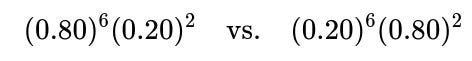
and multiply them by the respective priors 0.60 and 0.40, then normalize.
Performing the Calculation
Likelihood for hit:

Likelihood for miss:

Multiply them by the priors 0.60 (hit) and 0.40 (miss). Let’s illustrate how we might compute this directly in Python.
import math

prior_hit = 0.6
prior_miss = 0.4

like_hit = (0.8**6) * (0.2**2)
like_miss = (0.2**6) * (0.8**2)

numerator = prior_hit * like_hit
denominator = numerator + prior_miss * like_miss

posterior_hit = numerator / denominator

print(posterior_hit)
Running this (or doing it by hand) yields a posterior probability of approximately 0.9974. Interpreted in percentage terms, there is roughly a 99.74% chance that the show is a hit after observing that 6 out of 8 raters liked it.
Explanation of Why the Posterior is So High
Many find it surprising that the posterior probability ends up being around 99.7%. The reason is that an 80% like probability is quite high compared to 20%, so the likelihood ratio for 6 out of 8 in favor of the show heavily biases it toward “hit.” Specifically, 6 out of 8 likes is far more probable under a scenario where each viewer has an 80% chance of liking the show than if each viewer has only a 20% chance. Additionally, we began with a prior that already slightly favored “hit” (0.60 vs. 0.40). These factors compound to give a very strong posterior for “hit.”
Subtle Points to Consider
It’s important not only to plug in the numbers, but also to understand potential pitfalls in real-world data scenarios:
• Independence Assumption: We assumed the 8 in-house raters are independent in whether they like or dislike the show. In reality, raters might influence each other (e.g., if they watch the show together or share opinions), so the posterior might be less extreme if independence is violated.
• Prior Sensitivity: Changing the prior from 60% vs. 40% to something else (say 50% vs. 50%) or if you had strong reasons to believe the show is more/less likely to be a hit, the posterior would shift. However, the large likelihood difference can still drive the posterior heavily toward “hit.”
• Evidence Strength: Observing 6 of 8 likes is moderate evidence in favor of the show’s success. Yet, for a big difference in like probabilities (80% vs. 20%), even moderate evidence can become quite compelling in Bayesian terms.
What if Only 5 Out of 8 Liked It?
A natural follow-up question might be how the posterior changes if we had a slightly different outcome, like 5 out of 8 instead of 6 out of 8. Let’s answer that as well:
We simply use the same Bayesian formula but with the updated likelihood for 5 likes and 3 dislikes:
Likelihood for hit in that scenario:
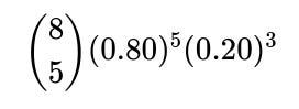
Likelihood for miss:

Both have the same binomial coefficient

, so after multiplying each by its prior (0.60 and 0.40 respectively) and normalizing, we would get a smaller posterior for “hit” compared to the 6 out of 8 scenario, but it would still likely favor “hit.” The exact number can be computed similarly.
Could the Posterior Probability Ever Decrease Below the Prior After Observing Some Likes?
A tricky question might be: “Is it ever possible that observing some likes actually reduces your belief in the show being a hit?” This could happen if we had so many likes that it was actually less probable under 80% than some alternative hypothesis that had an even higher like rate (though that’s not in our current problem). With only two hypotheses—80% chance of like vs. 20%—observing any pattern with more than 4 out of 8 likes will push the posterior more strongly toward the 80% side, since that pattern is more likely under the 80% model.
Deeper Insight Into Why the Ratio Is So Extreme
A standard way to grasp this is to look at the likelihood ratio between “hit” and “miss.” The ratio of the probabilities for 6 likes out of 8 is:

One can rewrite this as:

The term

is 4096. The term

is 0.0625. Multiplying them gives 256. This 256:1 likelihood ratio is enormous; once you also fold in the prior ratio of
0.60/0.40=1.5
you get 384. The posterior is
384/(1+384)≈0.9974.
Hence the large posterior.
Potential Pitfalls in Real-World Applications
Many interviewers will dig deeper into practical complications:
• Overfitting to Rater Feedback: Real watchers might differ systematically from in-house raters, leading to posterior overconfidence if the in-house ratings are not representative of the broader population.
• Beta-Binomial Conjugate Prior: If you had an underlying Beta prior for the “like” rate rather than a discrete hypothesis (hit vs. miss), you would do Bayesian updating on the continuous distribution. This can be more flexible but requires more advanced posterior calculations.
• Non-Binary or Contextual Aspects of “Like”: Sometimes a show might have partial likes, neutral opinions, or other forms of feedback not captured by a simple yes/no. This can complicate modeling and might require a more nuanced approach.
Regardless, in a simple discrete “hit vs. miss” scenario with independence and known probabilities of likes for each category, Bayesian updating with binomial likelihoods is straightforward. The final posterior of about 99.74% that the show is a hit indicates a very high belief after seeing 6 out of 8 raters liking it.
How Would One Implement This in a Real System?
A direct extension is:
• Define a discrete set of categories (e.g., “Likely a flop,” “Likely moderate,” “Likely a success,” “Likely a runaway hit”), each with a different prior and different probability of any individual liking the show. • As rater feedback arrives, multiply the prior for each category by the observed binomial likelihood, then normalize to get a new posterior distribution over categories. • Switch from discrete categories to a continuous prior, such as a Beta distribution for the “like” probability, so you can more flexibly handle uncertainty and update as more data comes in.
In standard data pipelines, you could keep a record of the number of likes and dislikes among internal screenings, then compute real-time posterior probabilities for different performance tiers.
Edge Cases: Very Few Raters or Very Many Raters
Another subtle area an interviewer might explore:
• If only 1 or 2 raters watched the show, the posterior might be highly sensitive and not very reliable. For example, if just 1 person rated it and they liked it, the posterior for “hit” would shift somewhat, but not too drastically because the data is meager. • If a very large number of raters have seen the show, the law of large numbers takes over. If the show’s true “like” probability is near 0.80, observing a proportion near 0.80 is highly likely, and your posterior that it is in fact a “hit” becomes extremely high, overshadowing the small chance that it’s a miss.
Conclusion of the Main Question
The posterior probability that the show is a hit, after observing 6 out of 8 raters like it, is approximately 99.74%. This result comes from the relatively large difference between the two likelihood models (80% vs. 20%) and the prior belief that already leans slightly in favor of “hit” (0.60).
Below are additional follow-up questions
How would you handle a scenario where each rater has a different probability of liking the show, rather than a single 80% or 20%?
In practice, not all raters are alike. Some might be more generous, and others more critical. The original calculation assumes a single fixed probability of liking (80% or 20%) across all 8 raters. If we suspect that each rater could have their own intrinsic bias, we need a different modeling approach.
A common technique is to assume each rater has a latent parameter that affects their likelihood of enjoying any given show. You could have a distribution over individual biases and then integrate out those biases in your Bayesian update. For a “hit” show, maybe the average like probability is high, but each rater’s personal taste might modulate that baseline probability. Similarly, for a “miss” show, you might have a low baseline that is again modulated by individual rater differences.
In a very simple extension, let

be the probability that rater
i
will like the show if it is a hit, and let

be the probability that rater
i
will like the show if it is a miss. To update the probability of the show being a hit, you would compute the product over all observed ratings:

where

is 1 if rater
i
liked it, and 0 otherwise. An analogous expression applies for “miss,” using

. With these likelihoods multiplied by the priors, you would normalize to get the posterior.
However, if the set of probabilities

and

is not known upfront, you may need a hierarchical Bayesian model to learn or infer them. This can become more computationally intensive, but it is often more realistic for real-world use cases.
A potential pitfall is overfitting the rater-specific probabilities if you have very few ratings per rater. In that case, you might place a prior on

and

(for instance, a Beta distribution) and do partial pooling to avoid extreme estimates. This ensures you do not become overconfident about a rater’s preferences based on too few data points.
How would the posterior change if we allow for correlations between raters’ opinions?
The standard binomial-based Bayesian approach relies on the independence assumption: each rater’s like or dislike is assumed independent given the show’s true status (hit or miss). But in many real settings, if a show receives a positive review from a respected rater, others might be influenced.
When ratings are correlated, the likelihood factorization that underlies the binomial expression no longer holds. If two or more raters have correlated opinions, you cannot simply multiply the probabilities independently. You must account for the joint distribution of the ratings.
A possible modeling approach for correlation is to assume a latent variable capturing “general sentiment” among raters. Then each rater’s response is partially driven by this shared sentiment. That might require specifying or learning the correlation structure, such as a covariance matrix in a multivariate probit or logistic framework. With 8 raters, a full correlation matrix has many parameters. More commonly, you might assume a single correlation parameter that captures a tendency for raters to move together.
A major pitfall is that naive models that ignore correlation will overestimate the certainty of the posterior. If most raters are in agreement (like in the scenario of 6 out of 8 liking the show), correlated models might find that it’s not as strong of an indicator if those raters were heavily influencing each other. This can reduce the posterior probability of the show being a hit compared to the simpler independent assumption.
How would you modify the approach if the show can be in more than two states, for example “blockbuster,” “moderate hit,” or “miss”?
When you expand beyond two discrete categories, you extend the same Bayesian logic but over multiple hypotheses. Let’s say there are three categories: “blockbuster” (e.g., 90% chance viewers like it), “moderate” (50% chance), and “miss” (20% chance). You also have a prior distribution over these three categories (for instance, 20%, 40%, 40%).
You would compute a likelihood for each category. For “blockbuster,” you use the probability that exactly 6 out of 8 liked it under a 90% success chance. For “moderate,” you use 50%, and for “miss,” 20%. Each is a binomial expression:

where

is the “like” probability for category

. Multiply by the respective prior and normalize among all three categories to get your posteriors. The main difference from the two-category scenario is that the denominator in the posterior expression extends to sum the products of prior and likelihood for all categories.
A subtle pitfall here is that you need good calibrations of these different “like” probabilities for each category, and good priors for how often each category occurs. If your categories are poorly defined or your priors are not realistic (e.g., you assume a 50% prior on “blockbuster”), you can end up with nonsensical posterior results. Always check your categories and calibrate them properly from historical data.
How could we incorporate the length or complexity of the show’s content into this Bayesian framework?
Sometimes, the probability a viewer likes a show might depend on factors like the show’s length or complexity. A short, easily digestible show might have a higher or lower probability of being liked than a longer, more niche show. The simple model we used is static: either 80% (hit) or 20% (miss). To incorporate show-specific characteristics, you can build a logistic regression or another parametric function that outputs the probability of a viewer liking the show given specific features: cast, genre, length, etc.
For instance, define a parameter

that captures the baseline log-odds of liking the show, plus additional parameters
for different features. Then for each rater, the probability of liking the show is computed as:

where
σ(⋅)
is the sigmoid (logistic) function. You can do Bayesian inference on these parameters if you have a prior on them, or you can do a maximum-likelihood approach first and then refine with a Bayesian update. The posterior probability that “the show will be liked by a random viewer” is then integrated or averaged over uncertain parameters.
A potential pitfall is over-parameterizing the model with too many show-specific features relative to the number of raters you have. If 8 raters watch a show with a large number of features in your logistic model, you might not have enough data to reliably learn each parameter. That can lead to wide posterior intervals and a less certain classification.
How would you address the situation where some raters only watched a partial cut of the show or were distracted?
If your 8 raters did not all watch the same final cut or some were not paying full attention, their decisions to like or dislike might differ systematically from that of typical viewers. In Bayesian terms, the “likelihood” part of your update is no longer purely about an 80% or 20% chance of liking the show; it might be 80% for raters who watch the full version but unknown (and probably lower) for partial watchers.
You can address this by splitting your raters into separate groups based on the conditions under which they watched the show, each with its own probability of liking. For instance, if half the raters watched the final version and half an early rough cut, you could model:
• Probability of liking the final cut if show is a hit: 0.80 • Probability of liking the early cut if show is a hit: maybe slightly lower, such as 0.70, if that rough cut is not as polished
Similarly for a miss scenario:
• Probability of liking the final cut if show is a miss: 0.20 • Probability of liking the early cut if show is a miss: maybe 0.15 or 0.25, depending on assumptions
You then multiply out the correct probabilities for each subgroup. The main pitfall is incorrectly assigning the probabilities for partial watchers. If you overestimate how close partial watchers’ experiences are to the final version, you might artificially inflate or deflate your posterior for “hit.” This is why in real production analytics, controlling or standardizing the environment is crucial.
How might the posterior probability shift if we had a significant marketing campaign influencing the raters?
If in-house raters are exposed to marketing hype or the show is heavily promoted, there is a psychological bias that might inflate the likelihood of them saying they “like” it. In Bayesian terms, this means that the observed 6 out of 8 likes might not directly correspond to a true 80% preference probability in the general population. Instead, it could be artificially inflated due to hype.
A way to handle this is to adjust your model or prior to reflect that rater opinions might be systematically higher than the true average. For example, if your marketing is particularly strong, you might guess that if the show is a “true hit” for the general population with a real like probability of 80%, your in-house group might like it at 85%. If the show is a “true miss” at 20%, your in-house group might still like it at 25%. These adjustments shift your likelihoods upward for the in-house raters, so your final posterior will be more conservative about calling it a hit for the general audience.
The major pitfall is quantifying how big this marketing effect is. If you guess incorrectly, your posterior could either be too high or too low. Gathering data from a small subset of raters who are not exposed to the hype can help calibrate these adjustments.
What if we want to incorporate the cost of misclassifying a miss as a hit and vice versa?
Up until now, we have treated the posterior probability as the final number we care about. However, in a real production scenario, the cost of taking a show to a large release if it’s truly a miss could be large, and the cost of rejecting a show that could be a hit is also significant. Bayesian decision theory tells us we should combine the posterior probabilities with the costs (or payoffs) associated with each decision (e.g., green-light the show for a big release, test it further, or shelve it).
After you have the posterior
P(Hit∣data)
, define a utility or cost function:
•
C(H_predicted=1,H_true=0)
is the cost of a false positive (promoting a show that is actually a miss). •
C(H_predicted=0,H_true=1)
is the cost of a false negative (not promoting a show that would have been a hit).
A rational decision would choose to promote the show if the expected cost of that decision is lower than the expected cost of rejecting it. Formally, compute the expected cost for “promote” vs. “reject”:

Whichever is smaller indicates the optimal decision in a Bayesian decision-theoretic sense. The main pitfall is that quantifying these costs can be challenging. Real-world cost estimates—marketing budgets, lost opportunities, brand damage—can be difficult to pin down with confidence, yet they critically change your decision threshold for calling something a “hit.”
How can the model be adapted if the probability of like for a miss show is not exactly 20%, but uncertain?
The original framing uses two fixed probabilities (80% for hit, 20% for miss). But what if the “miss” category includes a range of possible like probabilities anywhere from 0% to 40%? You can incorporate uncertainty into these probabilities by placing a prior over

and
. For instance, you might define:

Then, “hit” and “miss” become distributions rather than single points. If your prior knowledge says that a typical “hit” is around 80% but anywhere in 70%–90% range, you select hyperparameters

accordingly. Similarly, if a “miss” can vary from 0% to 40%, pick suitable hyperparameters for

Upon receiving data (like 6 out of 8 likes), you would update these Beta distributions. The new posterior is something that requires integrating over these distributions for

and

. This can be done with a small numerical approach or Markov Chain Monte Carlo if you want a more flexible framework.
A potential pitfall is computational complexity, as the two Beta distributions and the discrete category membership can lead to more elaborate calculations. Still, the payoff is a richer model that acknowledges that “80%” or “20%” might just be a rough guess, and you let the data refine that guess.
How do you handle the situation where only binary like/dislike data isn’t sufficient (e.g., if raters can provide a rating from 1 to 10)?
In many real rating systems, raters give a numeric score or a star rating rather than a simple like/dislike. That means your data is not Bernoulli but rather ordinal or continuous. The simplest extension is to treat the rating as coming from some distribution parameterized differently for a “hit” vs. a “miss.” For instance, for a “hit,” you might assume an average rating of 8 (out of 10) with some variance, and for a “miss,” an average rating of 3 with its own variance. Then you can compute the probability of each observed rating under each distribution and multiply them together.
Alternatively, if the rating is ordinal (like 1 star to 5 stars), you might use an ordinal regression model that ties the latent preference to thresholds in a cumulative distribution. The Bayesian update concept remains the same: you compute
P(Data∣Hit)
and
P(Data∣Miss)
using an appropriate likelihood for the rating type, multiply by the priors, and normalize to get your posterior for “hit” or “miss.”
A subtle pitfall is that numeric ratings often come with rater-specific calibration (some people rarely give 10/10, others often do), so you might need rater-specific intercepts or a hierarchical structure. If you ignore that, you might misinterpret the data and incorrectly push your posterior.
How would you proceed if you only get a fraction of the feedback sequentially (e.g., after each rater, you want to update the probability on the fly)?
Sequential updating is a hallmark of Bayesian methods: you do not need all 8 ratings at once. Suppose you have a prior of 0.60 for “hit” and 0.40 for “miss.” You observe the first rater’s response. You compute the posterior. Then the second rater’s response arrives, and you treat your new posterior as the prior for the next update. This continues until you have processed all 8.
Here is a simple code snippet demonstrating how to do it sequentially:
import math

# Let's say the data is a list of rater outcomes in order: 1 for like, 0 for dislike
# For example, the show receives: [1, 1, 0, 1, 1, 1, 0, 1]
# We'll see how the posterior evolves after each rater.

data = [1, 1, 0, 1, 1, 1, 0, 1]
p_hit = 0.6    # initial prior for 'hit'
p_miss = 0.4   # initial prior for 'miss'
like_if_hit = 0.8
like_if_miss = 0.2

for i, rating in enumerate(data, start=1):
    # rating = 1 => rater liked it, rating = 0 => rater disliked it
    # Compute the likelihood under hit
    if rating == 1:
        likelihood_hit = like_if_hit
        likelihood_miss = like_if_miss
    else:
        likelihood_hit = 1 - like_if_hit
        likelihood_miss = 1 - like_if_miss

    numerator = p_hit * likelihood_hit
    denominator = numerator + p_miss * likelihood_miss
    new_p_hit = numerator / denominator

    # p_miss is just 1 - p_hit in the 2-category scenario
    p_hit = new_p_hit
    p_miss = 1 - p_hit

    print(f"After rater {i} -> Posterior for hit: {p_hit:.4f}, miss: {p_miss:.4f}")
The advantage of this sequential approach is that you can stop gathering ratings early if you become sufficiently certain about the show’s status. Or conversely, if the data so far is inconclusive, you might choose to gather more raters. One pitfall is that, in practice, the order of raters might matter if there is potential correlation (e.g., people watch together or discuss among themselves). If you treat the ratings as conditionally independent but they’re not, your sequential updates might overstate your confidence.
How might you handle a scenario where the notion of “like” evolves over time as cultural tastes change?
Sometimes, a show that might be considered a hit today could be perceived differently if cultural preferences evolve. A comedic style, for example, might become outdated, reducing the probability that future raters enjoy it. In a longer-term approach, you might want a dynamic Bayesian model that updates not only on who has liked or disliked but also tracks how the probability of liking drifts over time.
For instance, you could define a time-dependent parameter

for “hit,” which might gradually shift according to a random walk or some specified process. Each new rating at time
t
updates your posterior on

. You might also have a prior for how quickly

can drift from one time point to the next. This is reminiscent of state-space models or Bayesian filters like the Kalman filter, except for a Bernoulli or binomial process.
The pitfall is increased model complexity: you must specify how quickly tastes can evolve and ensure you have enough data over time to credibly infer the drift. Otherwise, the model might behave erratically and shift

too freely, or it might be too rigid and fail to capture real changes in cultural tastes.