
ML Interview Q Series: Best Linear Prediction of Normal Variable Given Difference from Independent Normal Variable
Browse all the Probability Interview Questions here.
John and Pete are going to throw the discus in their very last turn at a champion game. The distances thrown by John and Pete are independent random variables D1 and D2 that are N(mu1, sigma1^2) and N(mu2, sigma2^2) distributed. What is the best linear prediction of the distance thrown by John given that the difference between the distances of the throws of John and Pete is d?
Short Compact solution
From the independence of D1 and D2, we have:
E(D1 - D2) = mu1 - mu2
Var(D1 - D2) = sigma1^2 + sigma2^2
Cov(D1 - D2, D1) = sigma1^2
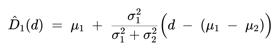
Therefore, the best linear predictor of D1 given D1 - D2 = d is
Comprehensive Explanation
Key Idea of Linear Prediction
The best linear predictor (or linear least squares estimate) of a random variable X given some observation Y generally takes the form X_hat = E(X) + [Cov(X, Y) / Var(Y)] [Y - E(Y)] assuming X and Y are jointly Gaussian or at least that we are focusing on linear predictors.
In this problem:
X corresponds to D1 (John’s throw).
Y corresponds to (D1 - D2).
Step-by-Step Derivation
1. Identify the Means
E(D1) = mu1
E(D2) = mu2
Since D1 and D2 are independent normal variables, we have: E(D1 - D2) = E(D1) - E(D2) = mu1 - mu2.
2. Compute the Covariance Cov(D1 - D2, D1) = Cov(D1, D1) - Cov(D2, D1).
Cov(D1, D1) = sigma1^2.
Because D1 and D2 are independent, Cov(D2, D1) = 0.
Hence, Cov(D1 - D2, D1) = sigma1^2.
3. Compute the Variance Var(D1 - D2) = Var(D1) + Var(D2) - 2 Cov(D1, D2). Because D1 and D2 are independent, Cov(D1, D2) = 0. Therefore: Var(D1 - D2) = sigma1^2 + sigma2^2.
4. Substitute into the Linear Predictor Formula Using the general form of the linear predictor, D1_hat = E(D1) + [Cov(D1 - D2, D1) / Var(D1 - D2)] [ (D1 - D2) - E(D1 - D2) ].
Plugging in the values:
E(D1) = mu1
Cov(D1 - D2, D1) = sigma1^2
Var(D1 - D2) = sigma1^2 + sigma2^2
E(D1 - D2) = mu1 - mu2
We get: D1_hat = mu1 + (sigma1^2 / (sigma1^2 + sigma2^2)) [ d - (mu1 - mu2) ], where d is the observed value of (D1 - D2).
Intuition Behind the Formula
The first term mu1 is the baseline (unconditional) expected distance for John’s throw.
The adjustment term (sigma1^2 / (sigma1^2 + sigma2^2)) [ d - (mu1 - mu2) ] corrects this baseline based on how different the observed difference d is from the expected difference (mu1 - mu2).
The ratio sigma1^2 / (sigma1^2 + sigma2^2) can be interpreted as the fraction of “confidence” we place on John’s own variance compared to the total variance of the difference.
Potential Follow-Up Questions
Why does independence simplify the covariance terms?
When two random variables X and Y are independent, it directly implies Cov(X, Y) = 0. In this scenario, that means Cov(D1, D2) = 0, thus Cov(D1 - D2, D1) becomes sigma1^2. If D1 and D2 were not independent (i.e., if there were some correlation ρ between them), we would need to incorporate that correlation in computing the covariance term.
What if the variables were not normally distributed?
For the best linear unbiased prediction (i.e., under the Gauss-Markov assumptions), normality is not strictly required for linear least squares estimates to be the best linear predictor. However, if the variables are not jointly Gaussian, then this linear predictor is not guaranteed to be the best in terms of minimizing mean squared error among all possible (nonlinear) predictors. It remains the best among all linear predictors, but not necessarily the best overall.
Could we interpret this result in terms of correlation coefficients?
Yes. The general form often uses the correlation coefficient ρ(X, Y). For two random variables X and Y,
X_hat = E(X) + ρ(X, Y) (σ_X / σ_Y) [ Y - E(Y) ].
In our setting, Y = D1 - D2, and X = D1. Because of independence of D1 and D2, the correlation between (D1 - D2) and D1 turns out to be
Cov(D1 - D2, D1) / [ sqrt(Var(D1 - D2)) sqrt(Var(D1)) ] = sigma1^2 / [ sqrt(sigma1^2 + sigma2^2) sigma1 ].
So the ratio that multiplies [ d - (mu1 - mu2 ) ] is essentially ρ(D1 - D2, D1) (sigma1 / sqrt(sigma1^2 + sigma2^2)).
How would you implement a quick simulation in Python to verify this?
Below is a simple demonstration. We can sample a large number of pairs (D1, D2) from their respective normal distributions, compute the difference d, then estimate D1 given d using the derived formula, and compare with the true value of D1 to see how well it performs:
import numpy as np

# Define parameters
mu1, sigma1 = 50.0, 5.0
mu2, sigma2 = 48.0, 5.0
N = 10_000_00  # number of samples

# Generate samples
D1_samples = np.random.normal(mu1, sigma1, N)
D2_samples = np.random.normal(mu2, sigma2, N)
diff_samples = D1_samples - D2_samples

# Compute best linear prediction for each observed difference
# \hat{D1}(d) = mu1 + (sigma1^2 / (sigma1^2 + sigma2^2)) * (d - (mu1 - mu2))
predictions = mu1 + (sigma1**2 / (sigma1**2 + sigma2**2)) * (diff_samples - (mu1 - mu2))

# Evaluate the mean squared error
mse = np.mean((predictions - D1_samples)**2)

print("Mean Squared Error of the linear predictor =", mse)
This code allows you to see how the derived formula performs in practice compared to the actual D1 values sampled. One would typically observe that this linear predictor yields the minimal mean squared error among all linear predictors.
What happens if sigma2^2 is extremely large compared to sigma1^2?
If sigma2^2 >> sigma1^2, the ratio sigma1^2 / (sigma1^2 + sigma2^2) becomes very small. Intuitively, that means Pete’s throw is extremely variable, so the observed difference d = D1 - D2 provides less reliable information about John’s actual distance. The formula will stay closer to mu1, ignoring the difference d to a large extent.
On the other hand, if sigma2^2 << sigma1^2, then the ratio becomes close to 1, indicating that the difference d is highly informative. We heavily adjust mu1 based on how far the observed difference is from its expectation.
How does this estimator relate to regression?
You can also view this problem through the lens of linear regression, where we want to regress D1 on the explanatory variable (D1 - D2). Given D1 = α + β (D1 - D2) + error, one can solve for α and β by the usual least squares method and obtain the same formula for β = Cov(D1 - D2, D1) / Var(D1 - D2) and α = E(D1) - β E(D1 - D2).
Thus, the best linear prediction is basically the fitted regression line for D1 against (D1 - D2).
Below are additional follow-up questions
What if the difference d is measured with some noise or measurement error?
If the observed difference between John’s and Pete’s throws is itself noisy (for instance, the measurement system introduces error so that the recorded difference is d_obs = (D1 - D2) + ε, where ε is an independent noise term), the best linear estimate must be adjusted to account for this added uncertainty. In such a scenario, the error term ε inflates the variance of the observed difference, so the weight we assign to the observed difference in estimating D1 should be smaller.
Concretely, we would replace Var(D1 - D2) = sigma1^2 + sigma2^2 with Var((D1 - D2) + ε) = sigma1^2 + sigma2^2 + Var(ε). The covariance Cov((D1 - D2) + ε, D1) would remain sigma1^2 if ε is independent of D1. The resulting linear predictor would place less confidence in the difference if measurement noise is large, pulling the estimate of D1 closer to its prior mean mu1.
This can be a subtle real-world issue if the measurement process is imperfect (e.g., a radar measurement with a known error variance). Failing to account for the measurement noise would make the model overly sensitive to fluctuations in the recorded difference and lead to higher variance in the estimate of D1.
How does this estimation change if we replace (D1 - D2) with (D2 - D1)?
If instead we observe d' = D2 - D1, then d' = - (D1 - D2). This sign flip simply modifies the mean we subtract in the predictor and changes the covariance sign accordingly. We would then compute E(d') = E(D2) - E(D1) = mu2 - mu1. The covariance Cov(d', D1) would be Cov(D2 - D1, D1) = - sigma1^2. Hence, the weight factor would introduce a negative sign, which flips the adjustment term in the best linear predictor.
Conceptually, since d' goes in the opposite direction of d, the predictor still yields the same numerical estimated value for D1—just with a sign change inside the bracket. The final expression would appear slightly different, but it would be algebraically equivalent once we substitute d' = - d.
Are there situations in which the best linear predictor might systematically under- or overestimate D1?
The linear predictor is unbiased if the assumptions are satisfied (i.e., if the model is correctly specified and the relationship is truly linear in terms of expectation). However, in real-world contexts:
If there is a systematic bias in measurement (for instance, if the measuring device systematically under-records Pete’s throw), then E(D1 - D2) might be off by a constant offset. This offset would cause a shift in how we interpret d, introducing bias into the estimate for D1.
If the distributions of D1 and D2 differ from the assumed Gaussians or if outliers occur frequently, the linear predictor can be less robust, sometimes leading to consistent over- or underestimation when the data are heavy-tailed.
To mitigate this, practitioners sometimes apply robust estimation methods or further correct for known systemic offsets.
What if we observe a truncated or censored version of the difference?
In some real competitions, we might only know whether John’s throw exceeded Pete’s throw by more than a certain threshold, or perhaps we only have partial information about the difference. For instance, we only learn that D1 - D2 > 0 if John’s throw is bigger, but not by how much. In such a case, the observable might be an indicator function I(D1 > D2) or a truncated difference.
The best linear predictor formula derived from the full difference no longer directly applies, because we do not observe the entire numeric difference. The best estimate in that scenario would generally require methods from truncated or censored data analysis—often involving more elaborate computations or Bayesian methods. The partial loss of information about the actual difference leads to larger uncertainty in estimating D1, and a purely linear approach might no longer be adequate without further assumptions.
How does the best linear predictor extend to more than two throwers?
Suppose now there are multiple throwers, D1, D2, D3, …, each with normal distributions (and possibly some correlation structure). If we wanted the best linear predictor of D1 given a set of differences such as (D1 - D2, D1 - D3, …), we would need to consider the vector of observations and the covariance matrix among all these variables. In matrix form, the best linear predictor becomes:
D1_hat = E(D1) + Σ_{D1, obs} Σ_{obs, obs}^{-1} (obs - E(obs)),
where obs = [(D1 - D2), (D1 - D3), …]. We would compute the block of covariances Σ_{D1, obs} and the block Σ_{obs, obs} using knowledge of Var(D1), Var(D2), Var(D3), etc., and their pairwise covariances. In other words, we are extending from a univariate difference to a multivariate regression problem. This highlights that the idea of “best linear predictor” generalizes naturally to higher dimensions, but the bookkeeping of covariance matrices becomes more involved.
Does knowing the sign of D2 or some additional partial observation about Pete’s throw change the estimator?
If, for example, we observe not only D1 - D2 = d but also a partial signal related to D2 (like an approximate measure of Pete’s throw or its sign above a threshold), that additional information can be exploited to form a different predictor. Because D1 and D2 are not correlated, the direct knowledge about D2 alone might not help estimate D1 unless it refines our knowledge of the difference more accurately (for example, if we combine an approximate measure of D2 with the difference to estimate D1). In practice, one could set up a joint distribution for (D1, D2) and incorporate any correlated piece of data (like partial observations about D2’s distribution). Even if the variables are marginally independent, certain observations of D2 might help reduce the variance of the difference measure d, depending on how the measurement or partial information is structured.
What happens if the variance of one thrower is extremely small compared to the other?
An extreme but different scenario from those previously mentioned is when sigma1^2 -> 0 for John’s throw, which means John’s throws are nearly constant at mu1. In that scenario, the best linear predictor effectively becomes “just take mu1,” because John’s throw barely fluctuates from its mean. Observing the difference d then doesn’t add meaningful information about a quantity that already has almost zero variance.
On the other hand, if Pete’s variance sigma2^2 -> 0, meaning Pete’s distance is almost always near mu2, then the difference (D1 - D2) is essentially (D1 - mu2). Observing that difference is then nearly identical to observing D1, and so the best linear prediction of D1 from (D1 - D2) = d is almost “just d + mu2.” This reveals how drastically the relative scale of these variances can affect how heavily the difference is weighted in estimating D1.
How might asymmetry in real-world throwing data affect the validity of the linear predictor?
While we assumed normality, real throwing data can sometimes be skewed (if, for instance, there is a physical limitation on how short or how far a throw can be). In such cases, the difference D1 - D2 might also have a distribution that deviates from a simple normal. Because the best linear predictor formula is derived under the assumption of joint normality (or at least independence and known variances), if the actual distribution is substantially asymmetric or heavy-tailed, the estimate can still be linear and unbiased but may no longer minimize mean squared error relative to a more carefully tailored nonlinear model.
Practically, one can either transform the data to approximate normality (e.g., using a log or power transform) or adopt robust regression approaches. If we suspect strong skewness, a log transform might be appropriate if all throws exceed some strictly positive threshold, though interpreting the difference of logs then becomes more complicated.
Is there a possibility that we want a predictor that is not linear?
In practice, the best linear predictor is not always the best predictor in terms of absolute or squared error, especially if the true relationship is nonlinear. For instance, if D1 is strongly bounded on one side and D2 is not, or if we had reason to believe that the relationship between D1 and (D1 - D2) is not linear, then a nonparametric or a more flexible parametric approach might yield lower prediction error.
A potential pitfall is overfitting if we bring in a more complex nonlinear model with limited data. The linear predictor is generally quite robust and easy to interpret. Hence, many real-world applications prefer the linear approach for its interpretability, unless there is strong evidence that a more complex function significantly improves predictive accuracy.
How would we test empirically whether this best linear predictor is well-calibrated in practice?
One approach is to gather a large dataset of actual throws (D1, D2). For each pair, compute the true difference diff_true = D1 - D2 and compare it to the best linear predictor’s estimate of D1 based on diff_true. We can plot predicted D1 versus actual D1 or compute the mean squared error of the predictions. We can also look at calibration metrics, such as whether the residual (actual D1 - predicted D1) has zero mean, or whether it shows any trend correlated with the observed difference. If we notice systematic drift in the residuals as diff_true increases or decreases, that is a sign the linear predictor might not be capturing some nonlinear pattern.
In real competitions or other physical processes, you might want to repeat this calibration step whenever conditions change (e.g., altitude, wind, new equipment) that could alter the distribution of the throws.