
ML Interview Q Series: Best-of-Seven Series Game 7 Probability: A Binomial Approach

Browse all the Probability Interview Questions here.
Consider a best-of-seven series between two teams, where each team has an equal 50% chance of winning any individual game. What is the probability that this series will require a seventh game?
Short solution from the snippet

Comprehensive Explanation
The probability that a best-of-seven series continues to a seventh game hinges on the exact scenario where neither side has already secured four wins in the first six games. Mathematically, that condition is equivalent to each team having won exactly three games each by the end of the sixth game. Because each team has a 50% chance of winning any single game, the probability framework relies on understanding binomial coefficients.
To see why the binomial coefficient enters the picture, think of the six games as a series of six independent Bernoulli trials for one team (for instance, “Team A wins” or “Team A loses”). We want the number of successful outcomes (Team A’s wins) to be exactly three. The number of ways to distribute three wins among six games is:

Since each game is a fair coin flip between two equally matched teams, the probability of any specific pattern of three wins and three losses is:

Multiplying the binomial coefficient by the probability of each arrangement gives:

Hence, the probability that the match goes to a seventh game is 5/16.

Below are further clarifications and additional details that often come up in interviews:
Reasons behind using the binomial coefficient. We only focus on splits of three wins for each side across the first six games, leading to a 3–3 scenario. That is exactly the way to ensure a seventh match occurs.
Importance of independence and equal win probability. The calculation relies on the fact that each game is independent of the others, with no advantage to either team. This independence and equal chance enable the simple binomial approach.
Implications for a general best-of-n scenario. If you had a best-of-n series (where n is odd), you could use the same reasoning. The probability of reaching the final game (game number n) can be computed by summing over the ways each team could split the first n−1 games evenly.
Simulating in Python. For completeness, a quick simulation can help confirm the theoretical probability.
import random

def simulate_series(num_simulations=10_000_000):
    go_to_game_7 = 0
    for _ in range(num_simulations):
        # Play up to 6 games
        teamA_wins = 0
        teamB_wins = 0
        for game in range(6):
            # Each game is 50-50
            if random.random() < 0.5:
                teamA_wins += 1
            else:
                teamB_wins += 1
        if teamA_wins == 3 and teamB_wins == 3:
            go_to_game_7 += 1
    return go_to_game_7 / num_simulations

prob_estimate = simulate_series()
print(prob_estimate)
Running such a simulation over a large number of trials should produce a figure very close to 5/16=0.3125.
What if one team has a different probability of winning each game?
If the probability of one team’s victory in each game was p instead of 0.5, the computation would involve a different binomial factor and the outcome would be:
to get to 3–3 after six games, followed by the seventh game. However, the question at hand specifically stated both teams have equal chances.
Could you double-check the result using a different reasoning approach?
Yes. Another approach is to list all possible sequences of six games and count manually how many sequences yield a 3–3 split, but that’s obviously cumbersome. Alternatively, you can apply the negative perspective, i.e., the series ends before game 7 only if one team reaches 4 wins in fewer than 7 games. Summing up probabilities of a 4–0, 4–1, or 4–2 outcome for either team can also be done. This method, after summation, will yield the complement probability of going to seven games, confirming 5/16.
Could we extend this logic to other scenarios in data science or machine learning?
In data science, we regularly encounter binomial probabilities and independence assumptions. The logic of counting ways something can occur and multiplying by the probability of each arrangement is fundamental to evaluating outcomes in Bernoulli processes (such as A/B tests, repeated trials, etc.). This problem highlights the value of combinatorial reasoning, which is integral to many ML and statistical methods, including hypothesis testing and designing simulations.
Is there a general takeaway for probability questions in interviews?
Interviewers are often interested in whether a candidate can break down problems into fundamental combinatorial blocks and apply the concepts of independence, binomial coefficients, and correct probability weighting. This particular example tests the candidate’s ability to handle combinatorial probability intuitively. It also offers an opportunity to demonstrate how to confirm analytical solutions through simulation, which is a useful approach in real-world ML settings when direct analytical solutions are more complicated or intractable.
Could you extend this result to find the probability that the series ends in 4, 5, 6, or 7 games?
One way is to recognize that for a best-of-seven, the series can end as soon as one team reaches four total wins. The probabilities for ending in exactly 4, 5, or 6 games can be found by applying binomial logic to the exact sequences where a particular team clinches the match on the final game of that set (and did not clinch earlier). For instance, for a series to end in 4 games, one team must win all four games in a row. You can sum the corresponding probabilities for both teams (since it could be either Team A or Team B).
Here is a breakdown of how one would handle each case:

What if the probability of winning each game is not 50%?
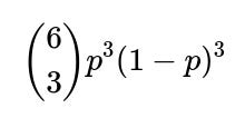
If Team A has probability p of winning any given game and Team B has probability 1−p, then the probability that the series goes to a seventh game follows the same binomial pattern but weighted by p and (1−p). Specifically, after six games, the event that each team is tied 3–3 has probability:

That quantity is how you would extend to an imbalanced scenario. In more complex real-world settings, p might even change from game to game (for instance, home-court advantage). In that case, you would need to multiply out different probabilities for each sequence rather than simply raising a single p to the number of wins.
How can we use a “negative approach” to verify the probability that the series goes to 7 games?
A negative approach sums the probabilities that the match ends in fewer than 7 games. Specifically, you look at the probability that one team wins in 4, 5, or 6 games, and then subtract that total from 1. If each team has an equal 50% chance per game, you can compute:
Probability that the series ends in exactly 4 games.
Probability that the series ends in exactly 5 games.
Probability that the series ends in exactly 6 games.
Summing those three probabilities and subtracting from 1 will confirm the probability that the series continues to the 7th game. It should match 5/16, providing a good consistency check on your answer.
How can we confirm our analytical result using simulation?
A quick Python simulation can estimate the probability empirically. You generate many simulated best-of-seven series. In each simulation, track Team A’s and Team B’s wins game by game until one reaches four total wins or until you have played six games. If after six games the teams are tied 3–3, count that simulation as one that goes to Game 7. At the end, divide the count of series that reached Game 7 by the total number of simulations. As the number of simulations grows large, this fraction converges to 5/16 when p=0.5. This approach is straightforward to implement and is invaluable for validating more complicated scenarios where a direct formula might be cumbersome.
Can we represent this problem with a state-based or Markov chain approach?
Yes. You could label states by a pair (i,j) indicating the number of wins for Team A and Team B, respectively. Each state transitions to (i+1,j) with probability p or to (i,j+1) with probability 1−p. The series terminates upon reaching any state where i=4 or j=4. To find the probability of specifically reaching state (3,3), you could sum up the transition probabilities leading to that state. Though it is more systematic, it ultimately yields the same binomial relationship we discussed.
How does this binomial logic appear in machine learning contexts?
In ML, we often deal with binomial distributions in hypothesis testing, A/B testing, or any setting involving repeated Bernoulli trials. The concept of counting “ways to have k successes in n trials” repeatedly arises. In classification tasks, you might measure how often a model predicts a positive class correctly, akin to a Bernoulli “success.” The mathematics of binomial coefficients helps you reason about variance, confidence intervals, and significance tests.
What if we wanted the distribution of all possible series lengths?
To get the distribution of lengths, note that the series can last 4, 5, 6, or 7 games. You can explicitly compute:
Probability of lasting exactly 4 games.
Probability of lasting exactly 5 games.
Probability of lasting exactly 6 games.
Probability of lasting exactly 7 games (which we already have as 5/16).
By summing these probabilities, you should get 1. This distribution reveals how likely it is for the series to be short (4 or 5 games) versus long (6 or 7 games). Such a question might come up if, for instance, you need to plan broadcasting schedules or estimate ticket revenues for potential home games.
How might the result change if a team gains a momentum advantage after consecutive wins?
If momentum changes the probabilities (e.g., after two consecutive wins, that team might have a higher chance of winning the next game), then the independence assumption breaks. One cannot use a simple binomial distribution because each game’s outcome depends on prior outcomes. Instead, you would need to build a Markov chain where the transition probabilities are conditioned on the sequence of recent results (for instance, a “state” might include the current scoreboard and whether the team is on a winning streak). This becomes more complex but is still systematically solvable, either analytically or through simulation.

How do you decide between using a closed-form formula versus a simulation in practice?
Closed-form formulas are exact, fast, and require fewer computational resources once you know the correct combinatorial or probability distribution. They also give you direct insight into the structure of the problem. However, deriving those formulas can be difficult if the problem is more intricate (e.g., not independent from game to game, not constant p). In such cases, simulation is a flexible alternative. Simulations let you incorporate any rule changes or complexities (such as momentum, varied probabilities per game, or other random effects) with relative ease. The trade-off is that simulations offer approximate answers and require enough runs to reduce sampling variance to acceptable levels.
By walking through these potential follow-ups, you prepare for how real interviewers might probe your depth of understanding, both for combinatorial probability basics and for applying these principles in more complicated or practical ML tasks.
How would you handle partial data if some outcomes are not equally likely?
Sometimes, real matches are not perfectly fair or the probability changes over time (injuries, changing strategies, home advantage, etc.). If you have partial data—for instance, a historical record of each team’s performance under certain conditions—you might estimate p empirically from that data. Or you could apply Bayesian methods that update a prior distribution on p based on observed wins and losses. In such a scenario, instead of a fixed p, you would integrate across the posterior distribution of p to arrive at a final probability. That approach is more advanced but aligns with how you might incorporate uncertainty in real-world forecasts or predictive models.
Expanded Explanation on Changing Probabilities and Empirical Estimation
In many real-world sports or competition scenarios, the assumption that each team has a fixed, unchanging probability of winning every game (like 50% vs. 50%) can be too simplistic. Several factors might cause the probability to shift from one game to the next:
Changing Team Strengths Due to Injuries: A key player might be injured or return from injury, altering the team’s effective strength. This situation introduces variability in the likelihood of winning, so the probability of victory could be different in Game 5 compared to Game 1.
Shifting Strategies: Coaches or teams often adjust tactics after observing how the opponent plays. If these adjustments significantly improve (or worsen) performance, the probability of winning is no longer the same for each game.
Home vs. Away Advantage: Many sports have pronounced home-field or home-court advantage. That means the probability p of winning at home might be higher than winning an away game, and this effect can flip when the venue changes.
Performance Slumps or Momentum: A team on a “hot streak” might perform better than expected, or a team in a slump might perform worse, so p could be larger or smaller depending on recent performance.

Below are ways to handle such partial or context-rich data:
1) Frequentist Estimation (Empirical Probability): Gather past matches that are “similar” (e.g., Team A at home against teams with a certain ranking). Let’s say the team won w times out of n matches in those similar conditions. Then an empirical estimate of the winning probability is p=w/n. This approach works well if you have enough historical data that closely resembles your current scenario. If data is sparse, you might combine multiple similar contexts or apply smoothing techniques (like adding a small “pseudo-count” in Bayesian terms).
2) Logistic Regression or Machine Learning Models: In more involved scenarios, you can build a classification model that predicts the outcome of a match based on various input features—home/away, recent performances, injuries, etc. The model outputs a probability of winning for the next game. Over time, you update or retrain the model as new data arrives. This approach handles more variables systematically.
3) Bayesian Updating: If you maintain a prior distribution on p (say, a Beta distribution) and observe new data (a few games and their outcomes), you can update your distribution to a posterior. This yields a refined estimate of p along with a measure of uncertainty. When you need to compute the probability of going to a game 7, you could integrate over your posterior distribution for p, effectively averaging all likely values of p.

Regardless of the specific method, the common theme is that you no longer assume a fixed 0.5 probability per game. Instead, you derive or learn the probability from the context and data available. If that data is “partial,” meaning you only have records of certain games, or your data is incomplete in describing conditions, you rely on estimation or modeling with the best information you have. This might involve taking fewer variables into account, making broader assumptions, or systematically modeling uncertainty.
In summary, while the textbook binomial approach works perfectly for a fixed “fair coin” scenario, real matches frequently demand a more nuanced model. In an interview setting, you’d emphasize that once the assumption of independence and identical probability (iid) is violated, you either look for a suitable distribution that fits the new scenario or rely on simulation/modeling techniques that incorporate the changing probabilities over time.