
ML Interview Q Series: Bias vs. Consistency: Understanding Critical Properties of Statistical Estimators

Browse all the Probability Interview Questions here.
4. What does it mean for an estimator to be unbiased? What about consistent? Give examples of an unbiased but not consistent estimator, as well as a biased but consistent estimator.
Understanding the Concepts
An estimator is a statistical method (often a function of sample data) that attempts to infer or approximate some parameter of the underlying distribution. Common parameters include the mean, variance, or more complex quantities depending on the problem.
Bias of an estimator is about how, on average, the estimator differs from the true parameter value across repeated samples.
Consistency of an estimator is about how, as the sample size grows large, the estimator converges (in some well-defined sense) to the true parameter value.
Below is a deeper discussion of each term, followed by detailed examples that illustrate how an estimator can be unbiased but not consistent, and vice versa.
Unbiasedness
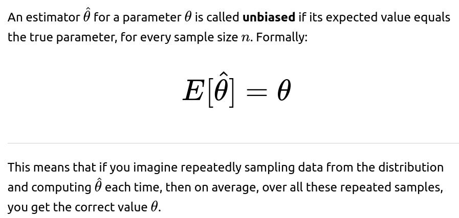
An unbiased estimator does not necessarily become more accurate as the sample size increases—it just means that on average it is correct. However, it might still have large variance in finite samples.
Consistency

Consistency does not necessarily imply unbiasedness in finite samples. An estimator can be slightly biased for small or moderate n, yet still converge to the true parameter as n grows large.
Example of Unbiased But Not Consistent Estimator
Key idea: You want an estimator that has the correct expectation but does not converge to the parameter as n grows. The reason it might fail to converge is often because its variance does not shrink as n increases.
A classic (though somewhat contrived) example is:

Example of Biased But Consistent Estimator
Key idea: You want an estimator that, for finite samples, has an expectation that differs from the true parameter value, but as n grows large, it converges to the true value.

Potential Follow-up Questions
What is the formal definition of consistency using convergence in probability?
Convergence in probability means that for every ϵ>0:
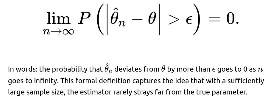
Follow-up considerations:
Sometimes people also talk about almost sure convergence or mean-square convergence. For consistency in the simplest sense, we usually focus on convergence in probability.
In an interview, you might be asked about whether “unbiased + large n” automatically implies consistency. The answer is no, because you could remain unbiased but still have a high variance that does not vanish with large n (as in the earlier example).
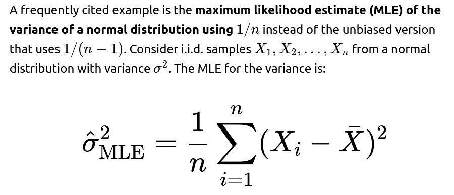
Why is the sample variance formula often written with 1/(n−1) instead of 1/n?
The sample variance with 1/(n−1) is called the unbiased estimator of the variance for an i.i.d. normal sample. It can be shown that:

When you use 1/n instead, you get the maximum likelihood estimator, which slightly underestimates the true variance on average, but that bias shrinks with n. Thus:
1/(n−1) version is unbiased and consistent.
1/n version is biased but consistent (the difference is negligible for large n).
Can an estimator be both biased and inconsistent?
Yes, there is no guarantee that a biased estimator must eventually converge to the true value. A biased estimator can fail to converge. For instance, you could define some pathological estimator whose bias increases or does not diminish with n. Or the estimator’s variance might grow, or some combination of bias and variance doesn’t allow it to approach the true value in probability.
How can an estimator be both unbiased and consistent?
Many standard estimators in classical statistics are both unbiased and consistent. For example:
The sample mean of i.i.d. data from a distribution with finite mean is both unbiased and consistent for the population mean.
The sample proportion (in a Bernoulli setting) is both unbiased for the true probability p and also consistent as the number of trials grows.

Are there scenarios where we prefer a biased but consistent estimator over an unbiased one?

Sometimes, an estimator might have a small bias but a significantly lower variance. As n grows, even that small bias disappears or becomes negligible, and the overall MSE might be smaller. Practitioners often choose consistent estimators with minimal MSE, even if there is a slight bias in finite samples.
Real-world example:
In regularized regression methods (like Ridge Regression or Lasso), the coefficients are typically biased toward zero, but the shrinkage often lowers variance and results in better generalization performance. These methods can still be consistent under certain conditions, though they are not unbiased.
Could you show a short Python example illustrating how we might empirically check bias or consistency?
Below is a simple Python code snippet that simulates a normal distribution and checks two estimators of the variance:
The 1/(n−1) version (unbiased and consistent).
The 1/n version (biased but consistent).
import numpy as np

def simulate_variance_estimators(num_simulations=100000, n=30, true_sigma=2.0, seed=42):
    np.random.seed(seed)
    # Generate samples from Normal(0, sigma^2)
    samples = np.random.normal(loc=0.0, scale=true_sigma, size=(num_simulations, n))

    # Unbiased estimator (1/(n-1)):
    sample_means = np.mean(samples, axis=1)
    unbiased_var_estimates = np.sum((samples - sample_means[:, None])**2, axis=1) / (n - 1)

    # Biased MLE estimator (1/n):
    mle_var_estimates = np.sum((samples - sample_means[:, None])**2, axis=1) / n

    return np.mean(unbiased_var_estimates), np.mean(mle_var_estimates)

if __name__ == "__main__":
    est_unbiased, est_mle = simulate_variance_estimators()
    print("Estimated mean of unbiased variance estimator:", est_unbiased)
    print("Estimated mean of biased MLE variance estimator:", est_mle)
Explanation:

Additional Follow-up Question: How do we formally relate bias and consistency to the Law of Large Numbers and the Central Limit Theorem?

These theorems illustrate the difference between an unbiased estimator (which might be correct on average but not necessarily tight) and a consistent estimator (which might be biased for small n but will converge in probability to the true parameter).
Additional Follow-up Question: Can an estimator be asymptotically unbiased but still consistent?
An estimator is asymptotically unbiased if:

Additional Follow-up Question: Are there practical reasons to choose a biased but consistent estimator?
Sometimes, yes. Reasons include:
Regularization: Introducing a small bias can drastically reduce variance, leading to better overall performance (lower MSE).
Computational simplicity: Certain biased estimators are easier to compute, especially in high-dimensional or complex settings, and the bias vanishes asymptotically.
Domain knowledge: In Bayesian statistics, introducing priors can cause small biases but often yields better performance if the prior information is well chosen.
Hence, the trade-off between bias and variance is at the heart of many practical machine learning and statistical modeling decisions.
Summary of Key Points

Biased but consistent example: MLE for variance with 1/n factor. Finite-sample expectation is off, but it converges to the true variance as sample size grows.
By focusing on mean squared error and asymptotic properties, one can see why, in practice, a biased but consistent estimator often suffices or may even be preferable in large-sample scenarios.
Below are additional follow-up questions
How do unbiasedness and consistency relate to the concept of minimum variance?
In classical estimation theory, we often hear about the “best unbiased estimator” or the “minimum variance unbiased estimator (MVUE).” This concept stems from the idea that among all unbiased estimators, we might prefer the one that has the smallest variance for each finite sample size. In other words, if an estimator is unbiased but has a large variance, it might be less desirable because its estimates could deviate significantly from the true parameter on a given sample, even though its average value over many samples coincides with the truth.
The Lehmann-Scheffé Theorem tells us that under certain regularity conditions, a complete sufficient statistic can be used to construct the UMVUE (Uniformly Minimum Variance Unbiased Estimator). This theorem highlights that not all unbiased estimators are equally good; some have lower variance than others. However, unbiasedness does not directly tell us about consistency. A minimum variance unbiased estimator is guaranteed (by definition) to have the lowest variance among all unbiased estimators for each sample size, but it could still, in theory, fail to be consistent if its variance does not shrink with n or some other subtlety arises.
In practice, especially in large-sample problems, we might prefer a slightly biased estimator that has lower variance and is consistent. For instance, maximum likelihood estimators in many scenarios are not unbiased for finite n but do have good large-sample properties such as consistency and asymptotic normality.
Edge cases to consider:
A scenario where a UMVUE might be extremely sensitive to outliers or high skewness, potentially making it undesirable in practice despite its unbiasedness and minimal variance among unbiased estimators.
Non-regular statistical models (e.g., distributions with infinite variance, heavy tails) where constructing a UMVUE is either impossible or leads to degenerate cases.
In summary, minimum variance among unbiased estimators does not automatically imply consistency. An estimator might be UMVUE yet have idiosyncrasies for particular sample sizes, especially if the underlying assumptions that guarantee certain properties are not met in real-world data. This is why advanced methods often trade off a bit of bias for higher stability.
Could there be real-world data situations where unbiasedness is irrelevant if the Mean Squared Error (MSE) is large?

Edge case scenarios:
High-dimensional settings: In high-dimensional regression or classification tasks, purely unbiased estimators can explode in variance. Regularization (which introduces bias) can drastically reduce variance and lead to better predictive performance.
Non-Gaussian heavy-tailed data: Outliers can heavily impact the sample mean (which is unbiased), causing extreme variance. A robust estimator (like the median) might be biased relative to the mean but has lower MSE because it is less sensitive to outliers.
In practice, MSE is usually the more relevant metric in real-world decision-making. If unbiasedness is a central concern (e.g., certain legal or financial applications where systematic misestimation is unacceptable), then bias is crucial. Otherwise, the MSE perspective typically drives practitioners to prefer methods that might be mildly biased but exhibit significantly less variance.
What if the estimator is consistent for a “trimmed” version of the parameter? Does that still count as consistent?
Sometimes, especially with heavy-tailed distributions, one might define a “trimmed mean” or a “robust estimate” that converges to a slightly modified version of the parameter. Strictly speaking, that estimator is consistent for the trimmed parameter, but it may not be consistent for the original theoretical parameter (like the raw population mean if the distribution has undefined moments or if the tails are so heavy that the classical mean is not meaningful).
In many practical applications, the “trimmed parameter” (like a 5% trimmed mean) is actually more reflective of what a practitioner wants to measure. That means:
The estimator is consistent for that robust target parameter.
It might be “biased” for the untrimmed mean parameter, but that untrimmed parameter could be ill-defined or not robustly estimable in the presence of outliers.
Edge cases:
Distributions where the mean does not exist, such as the Cauchy distribution. If one tries to estimate the mean of such a distribution with a classical estimator, it is ill-defined. A robust or trimmed approach could be more meaningful, even though it technically estimates a different quantity.
Data subject to heavy skew, where a 5% or 10% trimming might remove extreme outliers and yield more stable results.
Hence, calling an estimator “biased” or “unbiased” may lose some meaning if the underlying target parameter is changed. Always clarify what the parameter of interest is and whether it is well-defined or robustly estimable in the real-world scenario.
Why might the median be considered consistent for the population median but not unbiased for the population mean?
The sample median is a well-known robust estimator that estimates the population median. For i.i.d. data from a distribution with a well-defined median, the sample median will converge (in probability) to the true median. This makes the sample median a consistent estimator for the median of the distribution. However, if your parameter of interest is the mean, the median might be biased in most distributions (except symmetric ones like the normal distribution, where mean = median).
This raises the point that unbiasedness is always with respect to a specific parameter. If your parameter is the median, then the sample median is often unbiased (in certain distributions) or at least asymptotically unbiased and definitely consistent. But if your parameter is the mean, you can’t rely on the median being an unbiased estimator unless the distribution is symmetrical.
Edge cases:
Uniform distribution on [0, 1]: mean = 0.5, median = 0.5, so the sample median and sample mean converge to the same value, making the sample median effectively unbiased and consistent for that distribution’s mean.
Exponential distribution: mean = 1/λ, median = (ln(2))/λ. The sample median is consistent for the distribution’s median but is biased for the mean, and that bias does not vanish for small sample sizes. As n grows, the median estimate converges to the population median, not to the population mean.
Is maximum likelihood estimation always unbiased, and if not, does that affect its consistency?
Maximum likelihood estimators (MLEs) are not always unbiased. In fact, many popular MLEs (e.g., variance estimation of a normal distribution using 1/n) are biased in finite samples. However, the MLE often has strong asymptotic properties: under fairly general conditions, it is consistent and asymptotically efficient, and it converges in distribution to a normal random variable with variance given by the inverse of the Fisher information.
The fact that many MLEs are biased in finite samples rarely detracts from their usefulness. The primary reason is that the bias typically vanishes as n grows, or becomes negligible for large n. Moreover, the MLE can often be the simplest estimator to compute and reason about theoretically. In many real-world scenarios, the advantage of a conceptually straightforward and widely applicable method outweighs a slight finite-sample bias. If unbiasedness in small samples is critical, practitioners might apply a bias-correction, such as using 1/(n−1) in the sample variance estimate for the normal distribution or using more advanced bias-reduction techniques available for generalized linear models.
Edge cases:
Very small sample sizes: MLE might have significant bias. This can be critical in medical studies or scenarios with extremely limited data. In such cases, analysts might switch to unbiased or robust methods, or apply a Bayesian approach with strong priors.
Non-regular situations (e.g., distributions with undefined Fisher information, or boundary points in the parameter space): MLE can fail to be consistent or might be subject to different forms of bias that do not vanish as nn grows.
Is consistency guaranteed under the Central Limit Theorem (CLT), and what role does the CLT play in unbiasedness?
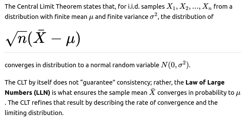
Regarding unbiasedness, the CLT doesn’t directly inform us whether an estimator is unbiased or not. What it does do is, if we start with an estimator that is consistent (like the sample mean) and also unbiased in finite samples, then the CLT can help us build confidence intervals and hypothesis tests around that estimator by telling us how it behaves for large n.
Edge cases:
If the data is not i.i.d. or if the variance is infinite, the standard CLT may not apply. In heavy-tailed distributions (like certain stable distributions), alternative limit theorems apply (e.g., Lévy stable laws), and standard consistency arguments for the mean might break down or require stronger assumptions (e.g., truncated data).
For time-series data with autocorrelation, the CLT might need to be replaced by a functional version or specialized results that account for dependence.
How can one handle bias that arises from model misspecification, and does that affect consistency?
Model misspecification occurs when the assumed form of the distribution or the functional relationship is incorrect. This can introduce systematic bias into estimators because they are effectively estimating a “best fit” within an incorrect model class, rather than the true parameter. For example, if you assume a linear regression model, but the true relationship is quadratic, the estimated linear slope might be biased for the real effect.
Such bias often does not vanish even as n goes to infinity, because no matter how large the sample, you are fitting the wrong functional form. This means the estimator could fail to be consistent for the true parameter. However, it might be consistent for the best linear approximation if we define a new parameter that is effectively the “slope in the best linear sense.”
Pitfalls:
Large sample sizes do not rescue you from a fundamentally incorrect model specification. This is a major real-world concern when modeling is done incorrectly or oversimplified.
Consistency is guaranteed under certain assumptions that the model form is correct (e.g., the standard linear regression model assumptions). Violate these assumptions significantly, and your estimator could converge to the wrong value.
To handle model misspecification, one might:
Use nonparametric or semiparametric approaches that place fewer structural assumptions on the data.
Conduct model diagnostics and residual checks to see if systematic patterns remain.
Use cross-validation or hold-out sets to test predictive performance, which can sometimes detect when a model systematically misses certain patterns.
In a Bayesian framework, how do we think about bias and consistency?
In Bayesian statistics, the concept of bias is less central because we combine a prior distribution with the likelihood to obtain a posterior distribution for the parameter. A point estimate, such as the posterior mean, might be biased from a frequentist perspective if we compare it to the true parameter across repeated samples from the “true” data-generating process. However, from a Bayesian viewpoint, that estimator is simply the expected value of the posterior.
Bayesian estimators can still be consistent under regular conditions. Typically, if the true parameter is within the support of the prior and certain regularity conditions hold, the posterior distribution will concentrate around the true parameter as n→∞. This means the posterior mean (or median, or mode) becomes consistent in a frequentist sense.
Pitfalls:
An overly informative or incorrect prior can induce significant bias that might not vanish quickly if the sample size is not large relative to the strength of the prior belief.
If the prior excludes the true parameter (has zero prior probability on that parameter), then no amount of data can correct that, and the estimator fails to be consistent.
Hence, from a Bayesian angle, “bias” is tied to prior assumptions. “Consistency” typically means the posterior distribution becomes sharply concentrated around the correct parameter as data accumulates, and this usually requires that the prior be reasonably well-behaved and not rule out the actual truth entirely.
Can measurement error or label noise turn an otherwise unbiased estimator into a biased or inconsistent one?
Yes, in practice, many measurement processes introduce extra noise or systematic errors that violate the assumptions that the data truly comes from the distribution we modeled. If the measurement error is random but has zero mean, you might still maintain unbiasedness in certain estimates, although the variance could grow. However, if the measurement error is systematically off (e.g., a sensor that always reads 5 units too high), that introduces additional bias in the observed data.
For consistency, if the measurement error is random and does not scale drastically with sample size, then under certain conditions the estimator can still be consistent for the underlying parameter because the law of large numbers may smooth out that additional noise. But if the measurement error is systematically correlated with the true values or grows with n in some complicated way, the estimator might no longer converge to the intended parameter.
Pitfalls:
In regression, “errors in variables” can lead to attenuation bias, where estimated coefficients shrink toward zero, and the problem does not vanish with large n because the bias stems from the correlation between regressor measurement error and the outcome.
In classification tasks, label noise that is systematically biased (some classes mislabeled more often than others) can skew training processes in a way that might not diminish with n. This can make certain estimates of accuracy or class probabilities inconsistent or heavily biased.
Hence, measurement error considerations are crucial in the design of data collection protocols and in the subsequent analysis. If the model incorrectly assumes there is no measurement error, the resulting inferences might be systematically off.
In model validation, how do we detect that an estimator is biased or inconsistent from practical diagnostics or data splitting?
In real-world projects, we often rely on techniques like cross-validation or out-of-sample tests to assess the performance of an estimator. While these methods do not directly prove unbiasedness or consistency, they can shed light on systematic deviations and how the estimator behaves with increasing amounts of data.
For instance, if you see that as you increase the training set size, the estimator’s predictions or parameter estimates remain systematically off even though variance shrinks, you might suspect a consistent bias. Conversely, if you notice the performance metrics keep improving and the estimate appears to get closer to the truth in repeated sampling or cross-validation folds, this suggests the estimator might be consistent (though not formally proven by these diagnostic checks alone).
Edge considerations:
Cross-validation distributions might still be noisy, especially if the data is not truly i.i.d. or if certain segments of data are not representative of the entire population.
Overfitting can mask whether an estimator is consistent. An over-parameterized model could appear to fit well on training data yet fail to generalize, implying no real convergence to the true parameter, especially if the model’s complexity grows with n.
Hence, in practice, we monitor both the bias (systematic offset in predictions or estimates) and the variance (fluctuations in estimates across different folds or subsets) to glean insights into whether the estimator might converge to the true parameter as data grows.