ML Interview Q Series: Biased Die Roll: Calculating Score Expectation and Variance with Probability Distributions

Browse all the Probability Interview Questions here.

A six‑sided die has four green faces and two red faces and is balanced so that each face is equally likely to come up. The die is rolled several times. We score 4 if the die shows green and 1 if it shows red. Let X be the score. Write down the probability distribution of X and calculate E(X) and Var(X).

Short Compact solution

The random variable X takes the value 1 with probability 1/3 (when the die shows red) and the value 4 with probability 2/3 (when the die shows green). Its expectation is 3, its second moment is 11, and its variance is 2. Concretely:

P(X=1) = 1/3

P(X=4) = 2/3

E(X) = 3

E(X^2) = 11

Var(X) = 2

Comprehensive Explanation

First, note that the die has 4 green faces out of 6 total faces, so the probability of rolling green is 4/6 = 2/3, while the probability of rolling red is 2/6 = 1/3. By definition of the random variable X:

• X=4 if the outcome is green

• X=1 if the outcome is red

Hence, we set P(X=4) = 2/3 and P(X=1) = 1/3.

To calculate the expectation, we use the general formula for the expected value of a discrete random variable. In plain text form, the expectation of X, denoted E(X), is the sum of all possible values of X multiplied by their respective probabilities.

In this problem, there are only two possible values of X, namely 1 and 4. Therefore:

E(X) = (1)(1/3) + (4)(2/3) = 1/3 + 8/3 = 9/3 = 3

Next, to calculate the variance, we often need E(X^2) (the expected value of X squared). The second moment E(X^2) is similarly computed by summing x^2 times p(x) over all possible x:

Substituting the two values of X:

E(X^2) = (1^2)(1/3) + (4^2)(2/3) = (1)(1/3) + (16)(2/3) = 1/3 + 32/3 = 33/3 = 11

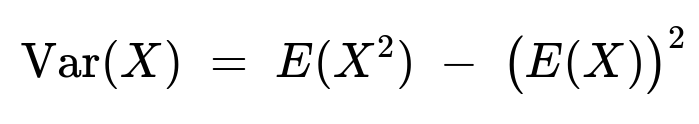
The variance of X is then obtained from the well‑known identity Var(X) = E(X^2) − [E(X)]^2:

Plugging in the values:

Var(X) = 11 − (3)^2 = 11 − 9 = 2

This confirms that the distribution of X is P(X=1)=1/3 and P(X=4)=2/3, with E(X)=3 and Var(X)=2.

A short Python snippet below shows how to empirically verify this through simulation:

import numpy as np

np.random.seed(42)

trials = 10_000_000
# X=4 with prob=2/3, X=1 with prob=1/3
X_samples = np.random.choice([1,4], size=trials, p=[1/3, 2/3])

empirical_mean = np.mean(X_samples)
empirical_variance = np.var(X_samples, ddof=0)  # population variance

print("Empirical Mean:", empirical_mean)
print("Empirical Variance:", empirical_variance)

As the number of trials grows large, the empirical mean should approach 3 and the empirical variance should approach 2, matching the exact theoretical values.

Follow‑up question: Why does E(X^2) matter when computing the variance?

Variance is defined as the expected value of (X − E(X))^2. Although one could compute this directly, it is almost always simpler to use the identity Var(X) = E(X^2) − [E(X)]^2. That is why E(X^2) naturally enters into the calculation of variance: it captures the expected value of the square of the random variable, which is crucial for measuring how spread‑out the distribution is.

In many practical machine learning settings, especially when dealing with Gaussian distributions or error measurements, second moments and variances are central to defining confidence intervals or loss functions (such as mean squared error). Therefore, one often deals with E(X^2) as a direct measure of the “average magnitude” of X.

Follow‑up question: What if the die was not balanced?

If the die were biased (i.e., not all faces are equally likely), we would need to carefully incorporate those modified probabilities into the calculation of E(X). For instance, if the probability of rolling green is p (not necessarily 2/3) and that of rolling red is 1 − p, then:

E(X) would be (4)(p) + (1)(1 − p).

E(X^2) would be (4^2)(p) + (1^2)(1 − p).

From those, we would again use the identity Var(X) = E(X^2) − [E(X)]^2 to find the variance. A bias would simply change the proportions in which the die shows green or red, but the methodology for calculating E(X) and Var(X) would stay the same.

Follow‑up question: How can we connect this to Bernoulli or binomial distributions?

Although X in this scenario takes values 1 and 4 (not just 0 and 1), we can sometimes transform the problem into a Bernoulli-like random variable by recentering or rescaling. If we define a Bernoulli variable Y that is 1 if the die is green and 0 if red, then Y ~ Bernoulli(p=2/3). In that case:

• E(Y) = 2/3

• Var(Y) = (2/3)(1/3) = 2/9

With X = 1 + 3Y, you can see that X is just a linear transformation of a Bernoulli random variable. In many machine learning tasks, recognizing such relationships (e.g., how one variable can be derived by shifting and scaling a Bernoulli outcome) helps simplify or reuse known distributions and properties.

Follow‑up question: Could we have computed variance by definition directly?

Yes. By definition, Var(X) = E[(X − E(X))^2]. You can compute this explicitly:

• With probability 1/3, X = 1, so X − E(X) = 1 − 3 = −2, and (X − E(X))^2 = 4

• With probability 2/3, X = 4, so X − E(X) = 4 − 3 = 1, and (X − E(X))^2 = 1

Thus E[(X − E(X))^2] = 4*(1/3) + 1*(2/3) = 4/3 + 2/3 = 6/3 = 2, exactly the same result as before. Both methods are valid, but using E(X^2) − [E(X)]^2 is typically more straightforward and less prone to arithmetic mistakes when the set of possible values of X grows larger.