ML Interview Q Series: Calculating Stockout Time & Lost Demand: A Poisson & Renewal-Reward Approach

Browse all the Probability Interview Questions here.

14E-13. Customers asking for a single product arrive according to a Poisson process with rate λ. Each customer asks for one unit of the product. Each demand which cannot be satisfied directly from stock on hand is lost. Opportunities to replenish the inventory occur according to a Poisson process with rate μ. This process is assumed to be independent of the demand process. For technical reasons, a replenishment can only be made when the inventory is zero. The inventory on hand is raised to the level Q each time a replenishment is done. Use the renewal-reward theorem to find:

a. The long-run fraction of time the system is out of stock. b. The long-run fraction of demand that is lost.

Verify that these two fractions are equal to each other.

Short Compact solution

In each cycle, the system is out of stock for an exponentially distributed time of mean 1/μ. The entire cycle length is the time out of stock (1/μ) plus the time it takes to go from Q units down to zero (Q/λ). Hence, the fraction of time the system is out of stock is:

The expected amount of demand lost in a single cycle is λ multiplied by the time out of stock (1/μ). Dividing by the total expected demand per cycle (λ times the entire cycle length), the fraction of demand that is lost is:

Because the Poisson process has the “Poisson arrivals see time averages” property, these two fractions are the same.

Comprehensive Explanation

Setup of the Problem

We have two independent Poisson processes:

• Demand arrivals: occurs at rate λ. Each arriving customer asks for 1 unit of the product.

• Replenishment opportunities: occurs at rate μ. A replenishment can only be performed if and only if the system is out of stock, and when it happens, the inventory level is instantly raised to Q units.

We lose any demand that arrives when the inventory is at zero (stockout). The key objective is to compute:

1. The long-run fraction of time that the system is out of stock.

2. The long-run fraction of demand that is lost.

3. Confirm that these two quantities coincide.

Regeneration Cycles

A “regenerative” cycle in this problem is defined as follows:

• Start of cycle: Immediately after an inventory replenishment event has restored the inventory to Q.

• End of cycle: The moment the inventory hits zero again (the next time it depletes to 0).

During each cycle:

1. We begin with Q units in stock.

2. Customers arrive one at a time (Poisson rate λ) and deplete the stock. Eventually, the stock hits zero.

3. Once the stock is zero, we wait for the next replenishment arrival (Poisson rate μ) to raise the stock from 0 to Q again, which ends the cycle and simultaneously begins the next one.

Hence, a cycle has two key time intervals:

• The time to go from Q units on hand down to 0. This is random but has an expected value Q/λ because the demand arrival process is Poisson(λ) and each customer consumes exactly one unit.

• The time spent waiting at zero until a replenishment event arrives. This waiting time is exponentially distributed with mean 1/μ.

Fraction of Time the System Is Out of Stock

Over a single cycle, the system is out of stock precisely during the waiting time for the replenishment event. That duration, call it T_out, is exponentially distributed with mean 1/μ. The length of the entire cycle, call it T_cycle, is T_out plus the time to go from Q to 0, whose expectation is Q/λ. Hence:

• Expected out-of-stock time per cycle = 1/μ.

• Expected cycle length = 1/μ + (Q/λ).

By the renewal-reward theorem, the long-run fraction of time the system is out of stock is:

where

• 1/μ is the average time out of stock per cycle (the “reward”),

• 1/μ + Q/λ is the average length of each cycle (the “renewal interval”).

Fraction of Demand That Is Lost

To find the fraction of demand that is lost, note that:

• The amount of demand lost in each cycle is simply the demand that arrives while the system is out of stock. Since the out-of-stock period in a cycle is an exponential interval of mean 1/μ, the expected number of arrivals during that interval is λ * (1/μ).

• The total demand in a single cycle is λ multiplied by the entire cycle length (since demand occurs at a constant rate λ).

Thus, the fraction of lost demand is:

1. Numerator: expected number of arrivals (demand) that arrive during the out-of-stock time, which is λ * (1/μ).

2. Denominator: total expected number of arrivals during the entire cycle, which is λ * (1/μ + Q/λ).

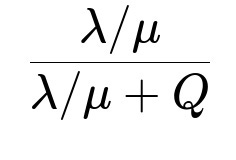
Canceling the factor λ from numerator and denominator yields:

Equivalence of the Two Fractions

Despite looking slightly different, these fractions are the same because:

• The fraction of time out of stock is (1/μ) / (1/μ + Q/λ).

• The fraction of lost demand is (λ/μ) / (λ/μ + Q).

We can see that if we multiply numerator and denominator of the fraction of time out of stock by λ, we get exactly the expression for the fraction of lost demand:

(1/μ) / (1/μ + Q/λ) × [λ/λ] = (λ/μ) / (λ/μ + Q).

Hence, they coincide. This highlights a well-known principle called “Poisson arrivals see time averages.” Since arrivals occur uniformly at random points in time, the fraction of arrivals that encounter a particular state (stockout) equals the fraction of time the system spends in that state.

Further Follow-Up Questions

What does “Poisson arrivals see time averages” mean in practical terms?

“Poisson arrivals see time averages” means that if arrivals occur according to a Poisson process and the system’s state evolves without influencing the arrival times, then from the perspective of arriving entities, the long-run proportion of arrivals that see the system in a given state is the same as the fraction of time the system actually spends in that state. In other words, under a Poisson arrival process, there is no bias toward arriving more often during certain conditions—arrivals are equally likely to appear at any random instant.

Why is the memoryless property so critical here?

Both the demand arrivals and the replenishment process are memoryless Poisson processes. The memoryless property implies that:

• The time until the next event (demand arrival or replenishment) does not depend on how long the system has already been waiting.

• After the inventory hits zero, waiting for a replenishment is an exponential random variable with mean 1/μ, making the cycle analysis straightforward.

• The time to go from Q to 0 is a gamma-type process if each arrival depletes one unit; however, its expectation Q/λ can be used in the renewal-reward setting.

Without these memoryless properties, the cycle analysis might become more involved, and the simple fraction-of-time and fraction-of-demand-lost formula would not be as clean.

What happens if Q = 0?

If Q = 0, then the system never actually has any stock after replenishment (because you “raise” the inventory to 0). The fraction of time out of stock is 1, since the system is always out of stock. Correspondingly, the fraction of lost demand is 1, meaning all demand is lost. This is a trivial edge case that the formulas confirm:

• Fraction of time out of stock = (1/μ) / (1/μ + 0/λ) = 1.

• Fraction of demand lost = (λ/μ) / (λ/μ + 0) = 1.

What if the arrival processes are not Poisson?

If arrivals are not Poisson, then the “Poisson arrivals see time averages” property may no longer hold. For instance, if arrivals happen in bursts or are scheduled at specific times, the fraction of demand lost could differ from the fraction of time out of stock. The renewal-reward theorem would still be applicable in some contexts, but deriving the exact expressions for these fractions might require more detailed analysis of inter-arrival distributions and scheduling.

How could one simulate this system in practice?

A simple Python simulation approach would be:

import numpy as np

def simulate_inventory(Q, lam, mu, n_cycles=10_000):
    np.random.seed(42)  # for reproducibility
    out_of_stock_time = 0.0
    total_time = 0.0
    lost_demand = 0
    total_demand = 0

    # Simulate cycles
    for _ in range(n_cycles):
        # Time to go from Q down to 0
        # We can approximate by generating Q exponential(1/lambda) inter-arrivals for demand:
        time_to_deplete = sum(np.random.exponential(1/lam, Q))
        total_time += time_to_deplete
        total_demand += lam * time_to_deplete  # expected arrivals in that period

        # Now system is out of stock
        # Time until replenishment
        time_wait = np.random.exponential(1/mu)
        out_of_stock_time += time_wait
        total_time += time_wait
        # Demand that arrives in that out_of_stock_time
        lost_during_wait = np.random.poisson(lam * time_wait)
        lost_demand += lost_during_wait
        total_demand += lam * time_wait

    return out_of_stock_time / total_time, lost_demand / total_demand

# Example usage:
frac_time_out, frac_demand_lost = simulate_inventory(Q=10, lam=2.0, mu=1.0, n_cycles=10000)
print("Fraction of time out of stock:", frac_time_out)
print("Fraction of demand lost:", frac_demand_lost)

• We track how long each cycle lasts, how much time we spend at zero inventory, how much demand arrives in total, and how much of it arrives while the system is out of stock.

• As n_cycles grows large, we expect the empirical estimates of the two fractions to converge.

In real deployments, you might structure the simulation differently or sample the depletions more precisely, but the principle remains the same: record time out of stock and total time, record lost demand and total demand.

Does the fraction of lost demand always match the fraction of time out of stock in real business settings?

In purely theoretical models with Poisson arrivals and exponential waiting times, yes, they match due to “Poisson arrivals see time averages.” However, in real-world applications:

• Demand may be non-Poisson (e.g., daily cycles, seasonal patterns, correlated arrivals).

• Lead times for replenishment may be deterministic or have different distributions rather than exponential.

• Practical constraints like order batching or a reorder policy with a lead time can complicate the standard renewal-reward approach.

Hence, while the equality holds for the simplified memoryless case, practitioners need to check whether assumptions remain valid in their specific operational environment.

Below are additional follow-up questions

How does the analysis change if partial replenishments are allowed before inventory reaches zero?

In the original setup, no replenishment can occur unless the stock level is exactly zero. Now imagine the system triggers a replenishment (raising inventory back to Q) whenever the inventory level falls below some threshold, say r > 0. This partial-replenishment scenario invalidates the simple “out-of-stock, wait for a replenishment” logic because there may be overlap between stock depletion and replenishment events. The renewal-reward argument no longer applies as straightforwardly, because the process is no longer neatly decomposed into cycles that start precisely at a full Q units and end at zero.

In practice, one would need to set up a more advanced continuous-time Markov chain (or semi-Markov chain if the interarrival times remain memoryless) to capture transitions between different inventory states. This typically involves:

• Defining the state by the current inventory level and whether a replenishment is in progress.

• Writing down the balance equations or using embedded Markov chain analysis at the times of arrivals/replenishments.

• Computing steady-state probabilities and using them to calculate performance measures like the fraction of time at zero stock or the fraction of demand lost.

A significant pitfall is that an intuitive “plug in partial replenishment” approach without carefully redefining the process states might lead to incorrect or oversimplified answers. In real-world supply chains, partial replenishment often complicates lead times, reorder points, and minimum order quantities, which further complicates the modeling.

How would results change if lost demand is backordered instead?

If lost demand is instead backordered, that means customers are willing to wait until a future replenishment arrives. The system does not lose demand but accumulates a backlog. Once the inventory is renewed, we fulfill the backlogged demand first, and only then is stock available to serve new arrivals immediately. This drastically changes the performance metrics:

• Instead of focusing on “fraction of demand lost,” we shift to metrics like average waiting time of customers, average backlog size, or fill rate over time.

• The fraction of time the system has no on-hand inventory might still be computed, but it is no longer the same as “fraction of demand that cannot be served.” In fact, if we never lose any customers, the fraction of demand lost is zero by definition, making it an uninteresting quantity.

• The time-average vs. arrival-average equivalence still holds for Poisson arrivals, but it would manifest differently, for instance in terms of the fraction of arrivals that must wait in backlog vs. those that find inventory immediately available.

The main pitfall is to assume you can just reuse the same renewal-reward analysis with a backordering system. In a backordering scenario, each cycle extends beyond hitting zero inventory because you continue to collect unfulfilled orders until the next replenishment. Analyzing that scenario typically involves queueing theory with infinite buffer capacity and an embedded Markov chain approach that tracks the backlog size.

Could correlated demand arrivals invalidate “Poisson arrivals see time averages”?

Yes. A crucial assumption in the property “Poisson arrivals see time averages” is that arrivals occur randomly in time with no correlation (i.e., the Poisson process is stationary and has independent increments). If arrivals become correlated—say, due to demand surges at certain times of day or seasonality patterns—then the system can spend more time in certain states exactly when arrivals happen to be more frequent or less frequent. This can lead to a discrepancy between fraction of time out of stock and fraction of arrivals encountering out-of-stock conditions.

For instance, if higher arrival rates tend to occur precisely when the system is likely to be out of stock, the fraction of demand lost can exceed the fraction of time out of stock. One common pitfall is ignoring daily or weekly cycles in demand. A real-world system with strong seasonality must consider these patterns; a purely Poisson-based analysis may underestimate lost demand during peak arrival times. Advanced approaches can include:

• Nonhomogeneous Poisson processes that allow time-varying arrival rates.

• Models of correlated interarrival times, e.g., via Hawkes processes (self-exciting processes) that capture bursts of arrivals.

What if replenishment times themselves are not memoryless?

The original problem assumes that replenishment events (opportunities to replenish) follow a Poisson process with rate μ, making each time to replenishment exponential with mean 1/μ once the system is out of stock. If replenishment opportunities follow some other distribution—for example, a deterministic schedule or a gamma distribution—then the memoryless property no longer holds. The renewal-reward setup can still be used, but only if the process remains regenerative in well-defined cycles.

• If the replenishment schedule is periodic (deterministic T time between replenishments), the cycle structure changes. You still get cycles from the point the system is replenished to the next time it hits zero, but out-of-stock intervals might not be exponentially distributed.

• If the time until the next replenishment has a general distribution, an embedded renewal approach is still possible, but you must carefully compute the expected out-of-stock interval per cycle and the expected length of each cycle with the correct distribution.

• A subtle pitfall is to confuse the independence of arrival events (demand) with the distribution of replenishment intervals. Even if they are still independent processes, non-exponential replenishment intervals can create “residual life” effects that make the time-average vs. arrival-average equivalence more complicated.

In more advanced cases, you may need to resort to a more general renewal-process framework or a Markov renewal process analysis to capture the distribution of cycle times accurately.

Does inventory level Q have to be an integer?

In many practical inventory models, Q is an integer, reflecting discrete product units. However, some theoretical treatments allow Q to be a continuous value, especially in large-scale supply chain approximations where partial units or aggregated demand are considered. If Q is not an integer:

• The times to go from Q to 0 might be modeled by fluid-flow approximations, where demand is subtracted continuously at some average rate λ. This is sometimes done in fluid queue models, leading to a deterministic depletion time of Q/λ if arrivals are treated as continuous flow.

• The renewal arguments still hold if you define a “cycle” as the time from a replenishment (stock raised to Q) down to zero. The fraction of time out of stock depends on the distribution of the time it takes to deplete Q units.

• A common pitfall is forgetting that partial units can complicate how actual orders are fulfilled if the arrival process is discrete. In real applications, we often keep Q integral for clarity, but fluid approximations can be helpful to gain insight into large-scale behavior.

How would you handle time-dependent rates (e.g., daily or seasonal effects)?

Time-dependent demand rates turn a stationary Poisson process with rate λ into a nonhomogeneous Poisson process with a time-varying rate λ(t). This invalidates the simple fraction-of-time vs. fraction-of-demand-lost equivalence derived from “Poisson arrivals see time averages,” because that property is specifically tied to stationary (constant-rate) Poisson processes. With a time-dependent rate, arrivals are more likely during some intervals. If the system is more likely to be out of stock at precisely those intervals, more arrivals will be lost.

One approach is to slice the timeline into small intervals where λ(t) is approximately constant, analyze each interval’s probability of being out of stock, and then aggregate results numerically or through simulation. Another approach is to perform discrete-event simulation with a time-varying arrival rate. A major pitfall is incorrectly applying the stationary Poisson logic to a non-stationary environment, leading to significant misestimations of lost demand or time out of stock.

Can blocking or concurrency in the replenishment process affect the result?

Sometimes, a system may not be able to replenish immediately when the inventory hits zero if another replenishment is “in progress,” or if there is a limit on how many replenishments can happen in a certain time frame. In such a scenario:

• You might have to queue replenishment requests themselves. Instead of a simple exponential waiting time with rate μ, you could face a queue for replenishment events with a certain service rate.

• The fraction of time out of stock may increase because you have an additional delay (waiting in the replenishment queue).

• The fraction of demand lost likely increases as well, because stock stays at zero for an extended interval while waiting for the queued replenishment to occur.

A common pitfall is to assume replenishments are always available “immediately upon hitting zero,” but in many real supply chains, there is a lead time or concurrency limit. Addressing this in the model requires queueing theory with more complicated states, possibly leading to a multi-dimensional Markov chain (tracking both inventory and the state of the replenishment queue).

How do you verify these analytical results against real-world data?

Verification typically involves collecting empirical data on:

1. Stock-out events: the timestamps at which the inventory hits zero, how long it stays zero, and how often replenishments actually occur.

2. Customer arrivals and lost sales: the frequency and timing of demand arrivals that encounter zero inventory.

You can then compute the empirically observed fraction of time out of stock (the total time at zero inventory divided by total observational time) and fraction of demand lost (lost units divided by total demand). One would compare these empirical estimates to theoretical predictions. Key pitfalls include:

• Data collection errors or delays, e.g., “shadow” demand that arrives but never even attempts to place an order because they see the product is out of stock.

• Seasonal or time-dependent arrivals that violate the stationarity assumptions.

• The presence of minimum order quantities or batching that modifies the replenishment times and volumes in ways the theoretical model does not capture.

Properly validating the model in production often reveals nuances like correlated arrivals, limited reorder concurrency, or partial backordering that were not accounted for in the original simplified theory.