
ML Interview Q Series: Calculating Poker Dealer Probabilities: Analyzing Bias in First Ace Selection.

Browse all the Probability Interview Questions here.
Question: In a poker game with three players A, B, and C, the dealer is chosen by the following procedure. In the order A, B, C, A, B, C, …, a card from a well-shuffled deck is dealt to each player until someone gets an ace. This first player receiving an ace gets to start the game as dealer. Do you think that everyone has an equal chance to become dealer?
Short Compact solution
We let p_k be the probability that the first ace appears at the k-th card. From basic conditional probability rules, it follows that p_1 = 4/52, p_2 = (48/52)*(4/51), and, in general, the expression for p_k is a product of the probabilities of not drawing an ace on all previous cards multiplied by the probability of drawing an ace on the k-th card. Numerically summing p_k across positions that correspond to each player's turn shows that r_A (the probability that A becomes the dealer) is about 0.3600, r_B is about 0.3328, and r_C is about 0.3072. Hence, not all three players have the same chance of becoming the dealer: r_A > r_B > r_C.
Comprehensive Explanation
Defining the probability p_k
We denote p_k as the probability that the first ace appears exactly at the k-th card in the entire dealing process (where cards are drawn one by one in the sequence A, B, C, A, B, C, …).
When dealing from a standard 52-card deck that contains 4 aces, the probability p_k can be obtained by ensuring that the first (k – 1) cards are all non-aces, and then the k-th card is an ace. The probability that the first card is not an ace is 48/52, the probability that the second card is not an ace (given that the first was not an ace) is 47/51, and so on, until the probability that the (k – 1)-th card is not an ace is (52 – (k – 2)) / (52 – (k – 2) + 1). Finally, the probability that the k-th card is an ace (given the first k – 1 cards contained no ace) is 4 / (52 – k + 1).
In large-font mathematical notation, we can write:
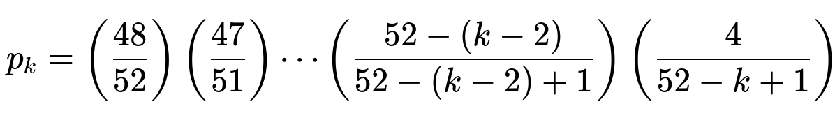
where k ranges from 1 up to 49 (in principle, there cannot be a “first ace” beyond the 49th card if the deck has 4 aces).
Determining each player's probability
The order of dealing is A, then B, then C, then A again, and so on. This means:
A gets cards 1, 4, 7, 10, … (3n + 1)
B gets cards 2, 5, 8, 11, … (3n + 2)
C gets cards 3, 6, 9, 12, … (3n + 3)
To find r_A (the probability that A is the first to get an ace), we sum p_k over all k in the form 1 + 3n (where n ranges from 0 until the index 1+3n exceeds 52). Similarly, we sum p_k over 2 + 3n to find r_B, and over 3 + 3n to find r_C.
These sums yield numerical probabilities:
r_A ≈ 0.3600
r_B ≈ 0.3328
r_C ≈ 0.3072
Why r_A > r_B > r_C
Because p_k is a decreasing function of k (it becomes less and less likely that no ace appears by a larger index k), the earliest “slots” in the dealing sequence are favored in terms of catching the first ace. Player A always occupies the earliest slot (card 1, then card 4, etc.) in each three-card cycle, so A benefits the most. B is second in each three-card cycle, and C is the last in each cycle, which explains why r_B and r_C follow r_A in descending order.
Practical intuition
Every time a trio of cards is dealt (one for A, one for B, one for C), if no ace has yet appeared, we move on to the next group of three cards in the same order. Because A “goes first” in each three-card group, the first ace that does appear is more likely to be in a position assigned to A. B has the second chance, and C has the third in each cycle, so their probabilities follow accordingly.
Potential Follow-up Questions
How can we verify the probabilities computationally?
A quick way to check or experiment with these probabilities is to simulate the dealing process many times and estimate the proportion of times each player ends up with the first ace.
import random

def simulate_first_ace_dealer(num_simulations=10_000_000):
    import math
    counts = {'A': 0, 'B': 0, 'C': 0}
    for _ in range(num_simulations):
        # Create a deck and shuffle
        deck = list(range(52))  # We'll let 0..3 represent the four aces, 4..51 represent non-aces
        random.shuffle(deck)

        # Deal in order A, B, C, ...
        player_order = ['A', 'B', 'C']
        card_index = 0
        while True:
            current_player = player_order[card_index % 3]
            current_card = deck[card_index]
            card_index += 1
            if current_card < 4:  # This means it is an ace
                counts[current_player] += 1
                break
    # Return approximate probabilities
    total = sum(counts.values())
    return {p: counts[p] / total for p in counts}

if __name__ == "__main__":
    results = simulate_first_ace_dealer(1000000)
    print(results)  # Should hover around {'A': 0.36, 'B': 0.33, 'C': 0.31}
By running such a simulation, we would empirically see that the results are close to the exact probabilities of about 0.36, 0.33, and 0.31.
Why is p_k decreasing in k?
As k increases, the event “first (k – 1) cards are not aces” requires a higher and higher number of consecutive non-aces in the deck. Since there are only 48 non-aces in the deck, the probability of seeing no aces in the first (k – 1) draws diminishes. Therefore, the chance that we make it all the way to the k-th card without encountering an ace keeps dropping, so p_k decreases with k.
What if the number of aces or players changes?
If there were more than 4 aces, then the probability distribution p_k changes to reflect that there are additional ways to draw an ace early. Each cycle still deals in the order A, B, C, but the probability of first seeing an ace at each position would be adjusted accordingly.
If there were only 2 players, a similar argument would show that the first player (the “A” seat) has an advantage because that position leads each 2-card cycle.
Could the positions ever be equal in probability?
If the deck had infinite size with infinitely many aces proportionally, or if the dealing order was changed each cycle, it might balance out. But with a finite deck and a fixed order, the first seat always gains an edge because they always receive the earliest draw in each cycle.
All of these points confirm that the procedure inherently favors the player who is first in the dealing rotation. Thus, it is conclusive that everyone does not have the same chance to become the dealer.
Below are additional follow-up questions
What happens if the deck is not a full 52-card deck?
If the deck is missing some unknown cards (for example, someone accidentally removed one or more cards before the game), the probability model changes. Instead of having 4 aces in 52 cards, there could be either fewer or the same number of aces in a smaller deck size. This scenario complicates the calculation in two ways:
We do not know how many non-aces are left if we do not know exactly which cards are missing. This introduces uncertainty into the probability of drawing an ace at each step.
Even if we did know precisely which cards are missing, we would need to recalculate the probability p_k by considering that the fraction of aces and non-aces in the smaller deck might be different.
A significant pitfall is that players might incorrectly assume the 4/52 ratio remains valid. If, for instance, a missing card happens to be an ace, then the real probability of drawing an ace early is actually lower than in the standard setup. Conversely, if the missing card is not an ace, then the probability of drawing an ace at each position is effectively a bit higher. In a real-world game, ensuring the deck is complete and correct is typically done to avoid these issues. But if the deck is tampered with or incomplete, the probabilities tilt unpredictably.
How does the reasoning change if we only have partial information about the remaining deck?
In some real-life situations, the dealer or the players might have seen some of the discards from a previous hand and thus have partial knowledge of which cards remain in the deck. If it is known, for instance, that one ace was discarded in an earlier round and that only certain subsets of cards remain, the probability analysis must incorporate that partial information. We then condition on the known cards that are no longer in the deck.
One major pitfall with partial information is incorrect or biased assumptions. If a player assumes that none of the aces have been removed when in reality one ace is gone, the entire probability distribution p_k is shifted. That mistaken assumption could lead a player to a false sense of security about how likely they are to draw the first ace. In formal terms, we would rewrite p_k with updated deck size and updated number of aces (for example, 3 aces out of 48 cards if we know some have been removed).
What if the dealing order itself changes unexpectedly during the procedure?
The mathematical derivation behind p_k assumes a strict repeating order: A, B, C, A, B, C, and so forth. If, for some unusual reason, the order changes mid-way—for example, if a house rule states that if a misdeal is suspected, the order restarts from B or C—this breaks the symmetry on which the standard analysis relies.
In that case, we would need to partition the event space according to the point in the sequence where the order changes. For instance:
If the order changes before any ace is drawn, we recalculate the probability that the first ace appears at some subsequent position k in the new order.
If an order change occurs after some cards have already been dealt without finding an ace, we combine the partial probability of getting that far with no ace and then continue with a different dealing sequence.
A subtle pitfall arises if players are not entirely sure when or how the dealing order might shift. That unpredictability introduces complexities in computing any closed-form solution. A simulation approach may be more feasible to estimate each player's chance.
How do we extend this logic if the same procedure is used for multiple consecutive deals?
Sometimes in casual poker games, players might decide that after one hand ends, the winner or some external factor determines who deals next. However, if they still elect to pick a dealer by looking for the first ace in the order A, B, C, and so on, for each new hand, then the advantage that the player in position A enjoys will compound over multiple hands.
Specifically:
If we independently repeat the “first ace selection” procedure each time a new dealer is needed, the probability that A ends up as dealer each time is still higher than for B or C on each new iteration.
Over many hands, A can expect to be the starting dealer more often, which might translate into a tangible game advantage if being the dealer offers strategic benefits (for instance, dealing last or having a special betting position).
The pitfall is assuming that the advantage “evens out” over multiple hands. Unless the order or the selection procedure is changed, the bias remains. In professional games, typically, dealer privileges rotate to ensure no one has this systematic advantage.
Can a player's strategy change the probability if they could choose not to draw?
In most standard poker dealing scenarios, players do not have an option to “skip” a deal. But hypothetically, if a house rule allowed a player to pass on receiving a card (effectively deferring to the next person in line), then the distribution of the first ace would change. Because p_k is decreasing in k, skipping a turn might or might not be advantageous, depending on how you expect the deck to evolve.
A bizarre edge case is that if skipping is allowed, one could game the system by deferring draws when the deck is more likely to produce an ace for the next person, hoping that it appears later on your next turn. However, since the deck is well-shuffled, it is not straightforward to exploit this consistently unless you have partial knowledge of which cards remain. The larger pitfall is that changing the order or skipping is not a standard poker rule, so most probability results do not apply without heavy modifications.
How might non-uniform shuffling or biased shuffling affect the outcome?
All of the derived probabilities rely on the assumption of a well-shuffled deck—meaning each arrangement of the deck’s 52 cards is equally likely. If the shuffle is biased (for instance, certain cards or positions are more likely to end up on top), the entire distribution p_k could shift. In an extreme case, if the deck were stacked by a magician or cheat to place an ace in a specific position, then a particular player could be almost guaranteed to receive the first ace.
A potential pitfall here is failing to detect cheating. If a player consistently notices that a certain seat is more likely to receive the first ace beyond the expected 0.36 vs. 0.33 vs. 0.31 split, it might indicate the shuffle is not truly random. From a theoretical standpoint, once you move away from uniform probability over all permutations, you lose the simple closed-form expressions for p_k. Instead, the distribution would depend on the exact nature of the shuffle bias.
What if each player is assigned multiple seats in the sequence?
Imagine a strange modification where A, B, and C do not each just occupy one position in the 3-step cycle but perhaps have multiple seats—for instance, if a single person is effectively playing as two “virtual players” in the rotation. Then that single person might get the 1st and 3rd positions in each cycle, while the others get the 2nd and 4th positions, or some other arrangement.
This scenario is unrealistic in standard poker, but conceptually it is interesting. We would define positions 1, 2, 3, 4, … in the sequence and see which person(s) they correspond to. The probability that a given person receives the first ace is then the sum of p_k over all k that belong to that person’s positions. If one individual has earlier or more frequent positions, their probability rises. A major pitfall is that you might incorrectly treat each “virtual seat” as separate in the sense of the deck’s run of cards, without properly summing probabilities for all seats that belong to the same player.
How does the result change if we add more special cards, like Jokers or wild cards?
Some poker variants add Jokers or use wild cards (sometimes even multiple). If we consider the “ace selection” procedure to stop when the first “ace or Joker” is drawn, we must recalculate the probabilities because we effectively have more than 4 “special” cards that can trigger the stop condition. For instance, if there are 2 Jokers, we have 4 aces plus 2 Jokers, for a total of 6 “stop” cards.
In that modified scenario, the probability that the first special card appears on the k-th draw is computed similarly but now the probability of “not drawing a special card” changes to (52 – 6)/52 for the first card, (51 – 6)/51 for the second, and so forth (assuming none of the special cards have been drawn yet). As before, summing over all k positions that belong to each player yields each player’s probability. Because the first player in the order still gets the earliest shot each round, they continue to have an advantage. The pitfall is to erroneously treat the situation exactly like the 4-ace scenario if you forget to incorporate the additional special cards.