
ML Interview Q Series: Calculating Circle Circumference Probability using Double Integration of Joint PDF x+y

Browse all the Probability Interview Questions here.
11E-9. The joint density function of the random variables X and Y is given by

Consider the circle centered at the origin and passing through the point (X,Y). What is the probability that the circumference of the circle is no more than 2π?
Short Compact solution
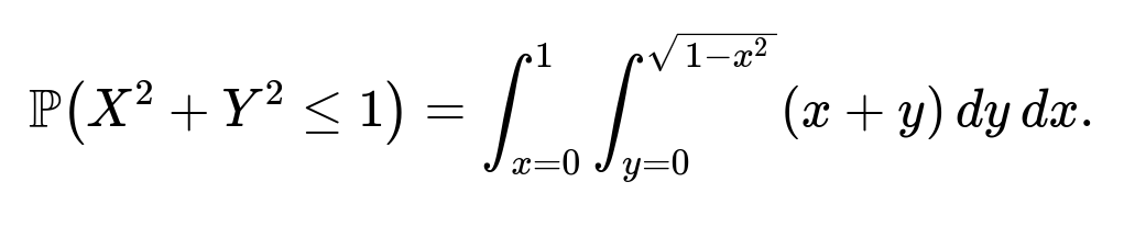
Because the circumference of the circle passing through (X,Y) is 2π√(X² + Y²), the condition “no more than 2π” is equivalent to √(X² + Y²) ≤ 1, so we need P(X² + Y² ≤ 1). We integrate x + y over the quarter of the unit disk where 0 ≤ x ≤ 1 and 0 ≤ y ≤ √(1 − x²). Performing this double integral yields 2/3.
Comprehensive Explanation
Interpretation of the problem
We have two random variables X and Y defined on the unit square [0,1] × [0,1] with a joint probability density function (pdf) f(x,y) = x + y. We are asked to find the probability that the circumference of the circle (centered at the origin) passing through (X,Y) does not exceed 2π. The circumference of such a circle is 2π times its radius, and the radius is simply the distance from (0,0) to (X,Y), which is √(X² + Y²).
Hence the inequality “circumference ≤ 2π” translates to:
circumference = 2π√(X² + Y²) ≤ 2π ⇒ √(X² + Y²) ≤ 1 ⇒ X² + Y² ≤ 1.
Thus, the event {circumference ≤ 2π} is equivalent to {(X,Y) falls within or on the unit circle centered at the origin}. Since X and Y only take values in [0,1], we are effectively restricting our attention to the quarter circle in the first quadrant.
Setting up the integral
We want the probability:
Here, 0 ≤ x ≤ 1 restricts us to the vertical strip along the x-axis from 0 to 1, and for each such x, 0 ≤ y ≤ √(1 − x²) keeps us inside the quarter of the unit circle.
Evaluating the integral
Inner integral over y: For a fixed x in [0,1], integrate (x + y) with respect to y from 0 to √(1 − x²):
∫(from y=0 to y=√(1 − x²)) (x + y) dy = ∫(from y=0 to y=√(1 − x²)) x dy + ∫(from y=0 to y=√(1 − x²)) y dy = x · [y] (from 0 to √(1 − x²)) + (1/2) · [y²] (from 0 to √(1 − x²)) = x·√(1 − x²) + 1/2( (√(1 − x²))² ) = x√(1 − x²) + 1/2(1 − x²).
Outer integral over x: We now integrate that expression with respect to x from 0 to 1:
∫(from x=0 to x=1) [ x√(1 − x²) + (1/2)(1 − x²) ] dx.
This can be separated into two integrals:
∫(0 to 1) x√(1 − x²) dx + (1/2) ∫(0 to 1) (1 − x²) dx.
For ∫(0 to 1) x√(1 − x²) dx, one may use the substitution u = 1 − x². After computing carefully, the result is 1/3.
For (1/2) ∫(0 to 1) (1 − x²) dx, it is (1/2)[ x − x³/3 ] from 0 to 1 = (1/2)(1 − 1/3) = (1/2)(2/3) = 1/3.
Summing these results 1/3 + 1/3 = 2/3.
Hence,

This completes the probability calculation.
Why the region is only in the first quadrant
Because the pdf f(x,y) = x + y is explicitly stated to be 0 for x or y outside [0,1]. Even though the circle is centered at the origin in the full plane, the only area that contributes to the probability is the portion of that circle lying within the unit square in the first quadrant.
Checking that f(x,y) is a valid pdf
A quick check for validity of a pdf requires verifying
∫(x=0 to 1) ∫(y=0 to 1) (x + y) dy dx = 1.
This indeed evaluates to 1, confirming that f(x,y) is a valid density function over [0,1]×[0,1].
Possible Follow-Up Questions
1) Could (X,Y) lie outside the quarter circle if X or Y is negative?
No. By definition of this particular pdf, both X and Y lie in [0,1]. Therefore, negative coordinates are impossible for this random pair, and we remain in the first quadrant.
2) How do we confirm that X² + Y² ≤ 1 corresponds to the event we need?
The circle’s circumference is 2π times the radius. The radius is the distance from the origin to (X,Y), which is √(X² + Y²). So 2π√(X² + Y²) ≤ 2π is satisfied exactly when √(X² + Y²) ≤ 1.
3) Is there a geometric interpretation for the 2/3 result?
Yes. The joint pdf places higher density the farther (x,y) are from (0,0) along either axis because it grows linearly with x and y. Hence, we weight points near (1,1) more strongly. Even though the region X² + Y² ≤ 1 is the quarter unit disk, the factor (x + y) shapes the probability in such a way that the final answer is 2/3, rather than the area ratio (which would have been π/4 if the density were uniform).
4) Could this be computed via simulation?
Yes. One could generate samples (X,Y) in [0,1]² with probability density proportional to x + y. To do that in practice, you might use rejection sampling or transform methods. Then approximate the fraction of points for which X² + Y² ≤ 1. As the number of samples grows large, the empirical fraction should converge to 2/3.
5) What if we wanted the expected value of X + Y given X² + Y² ≤ 1?
We could use conditional expectations and integrals. The approach would be:
Compute the numerator: ∫ over the quarter circle of (x + y)(x + y) dy dx.
Then divide by the probability 2/3.
This would be a straightforward extension, although more algebraic work would be involved.
All these discussions highlight how to set up and compute double integrals of different forms and verify that one correctly interprets the probability region under a non-uniform density.
Below are additional follow-up questions
1) What if the density function were slightly different, for example f(x, y) = c(x + y) with c chosen so that the total integrates to 1?
If we had a modified density f(x, y) = c(x + y), for x in [0,1], y in [0,1], then we would need to find the constant c such that
∫(0 to 1) ∫(0 to 1) (x + y) dy dx = 1/c.
In fact, for the original problem, c = 1 because:
∫(0 to 1) ∫(0 to 1) (x + y) dy dx = 1.
If c were different, say c ≠ 1, we would have
∫(0 to 1) ∫(0 to 1) c(x + y) dy dx = c ∫(0 to 1) ∫(0 to 1) (x + y) dy dx.
We would solve for c so that the integral equals 1. After determining c, we would then compute the same probability P(X² + Y² ≤ 1) by integrating c(x + y) over the region {x² + y² ≤ 1, 0 ≤ x ≤ 1, 0 ≤ y ≤ 1}. The only step that changes is the constant factor c in front of the integrand. The resulting probability would be the same fraction if we end up normalizing to 1 over [0,1]×[0,1], but we have to be consistent with the correct normalization constant to ensure that f(x, y) remains a valid pdf.
A subtle pitfall is forgetting to normalize properly. If you forgot to adjust c so that ∫ f(x,y) = 1, the entire probability calculation for events like X² + Y² ≤ 1 would be off by a constant factor. Also, if c turned out to be negative or zero for some reason, that would violate the nonnegativity condition of a pdf. It is critical to check that c > 0.
2) How could we approach the integration using a direct geometry argument rather than standard Cartesian integrals?
One might consider a geometric viewpoint if the pdf were uniform. For a uniform pdf over [0,1]×[0,1], the probability of an event is the ratio of the event’s area to the total area of the square. Here, however, the pdf is not uniform; it is weighted by (x + y). A pitfall is to mistake the probability for the ratio of areas, which would be π/4 for the quarter unit disk over the unit square. That logic would fail here because points near (1,1) are given a higher density.
If we wanted a “geometric-like” argument, we would need to consider that each point in the square is weighted by x + y. We could imagine slicing the region into infinitesimal strips and weighting each by the density. But that’s essentially replicating the Cartesian integral in a more intuitive “summing slices” approach. The key pitfall is incorrectly trying to apply an “area-based ratio” approach when the pdf is not uniform.
3) What if the region of interest were X² + Y² ≤ r² for some r < 1? How does the answer change?
When r < 1, we would look at the event {X² + Y² ≤ r²} in the first quadrant. We would still integrate (x + y) over x from 0 to r, and y from 0 to √(r² − x²). The integration method is analogous:
∫(x=0 to r) ∫(y=0 to √(r² − x²)) (x + y) dy dx.
A subtlety arises if r > 1, because the region X² + Y² ≤ r² might extend beyond the unit square. But if r ≤ 1, the quarter circle is entirely within the square, so the integral is straightforward. For r > 1, the region in question covers more than just the quarter disk in the square, but the pdf is zero beyond x=1 or y=1, so effectively the region stops at the square’s boundaries. A major pitfall is forgetting to cap x and y at 1. If r > √2, for instance, that circle extends well beyond the square, but the pdf is zero outside x>1 or y>1, so the actual integration region is the full unit square in that scenario.
4) Could we evaluate the same probability by converting the integrand to polar coordinates?
It’s tempting to switch to polar coordinates for a region defined by a circle, since X² + Y² ≤ 1 might look simpler. However, the pdf f(x, y) = x + y in polar coordinates becomes r cos(θ) + r sin(θ). The bounds for the region also become somewhat tricky because we only integrate over θ in [0, π/2] (the first quadrant) and r in [0,1]. Hence, the probability becomes:
∫(θ=0 to π/2) ∫(r=0 to 1) [r cos(θ) + r sin(θ)] r dr dθ.
This r outside is from the Jacobian of polar coordinates. One pitfall is to forget the extra factor r from the determinant of the Jacobian transformation, leading to an incorrect integral. Another subtlety is ensuring the angle range is correct. If we included [0,2π], we would be covering the entire circle, but we only want the quarter in the first quadrant because X, Y ∈ [0,1]. So the correct θ range is [0, π/2]. If you get that range wrong, you’d double, triple, or quadruple the integral, leading to a completely incorrect answer.
5) Does the problem change if we consider the boundary case X=0 or Y=0 specifically?
Because the pdf is (x + y) in [0,1]×[0,1], at X=0 or Y=0, the density reduces to y or x respectively. These boundary lines are perfectly valid subsets of the domain. However, in continuous distributions, the probability of landing exactly on a boundary line (like X=0 or Y=0) is zero in terms of measure. Thus it doesn’t affect the integral-based probability. A potential pitfall is to think that having X=0 or Y=0 might exclude or alter the region in a meaningful way for the integral. But line boundaries in 2D have zero area, so they do not affect the final numeric probability.
6) Could numerical integration methods pose any issues in computing this probability in practice?
If someone tries to compute
∫(0 to 1) ∫(0 to √(1 − x²)) (x + y) dy dx
numerically (e.g., using Riemann sums, Monte Carlo, or trapezoidal integration), the shape of the boundary y = √(1 − x²) can lead to error if the step size is large or the sampling method is naive. A direct pitfall is incorrectly discretizing the boundary or using too coarse a grid near the curved edge, which can produce a biased approximation. Also, if implementing a Monte Carlo method, one must ensure points (x, y) are sampled proportionally to (x + y), which is not trivial. Rejection sampling might be needed, and if not done carefully, the user might mis-sample. These are standard pitfalls in numerical approximation—especially when a nonuniform pdf complicates how random points are drawn.
7) How would the answer be affected if the circle were centered at (a, b) ≠ (0, 0) instead of the origin?
The circle passing through (X, Y) is now centered at (a, b). Its radius would be the distance from (a, b) to (X, Y). The condition “circumference ≤ 2π” translates to:
2π √((X − a)² + (Y − b)²) ≤ 2π,
which simplifies to √((X − a)² + (Y − b)²) ≤ 1. That is the event {(X, Y): (X − a)² + (Y − b)² ≤ 1}. We still only integrate over the unit square [0, 1] × [0, 1]. The difference is that the region might not even intersect parts of the square or it might intersect in complicated arcs if (a, b) is far from the square. Pitfalls include:
If (a, b) is outside the unit square, the circle might partially overlap or not overlap at all.
The integrand x + y remains the same, but the boundary region is now more complicated to describe in Cartesian coordinates.
We must carefully determine the intersection of (X − a)² + (Y − b)² ≤ 1 with 0 ≤ X ≤ 1, 0 ≤ Y ≤ 1.
Hence, the integral setup can become more involved, and it’s easy to make mistakes describing the domain. One might resort to geometric splitting or parametric forms to handle the partial arc within the square.
8) Suppose we were to compare the probability that X² + Y² ≤ 1 to a simpler or more complicated event. How can we ensure correctness?
When verifying a more complicated event, it helps to:
Break the region into simpler subregions if the boundary is piecewise.
Use well-tested transformations (like polar coordinates) but be mindful of the correct bounds.
Check corner cases where the region might be entirely inside or outside the square. For instance, if the event was X² + Y² ≤ 0.5, that region is entirely inside the first quadrant portion of the circle, but if we asked X² + Y² ≤ 2, that circle might exceed [0,1]×[0,1].
A consistent pitfall is incorrectly handling partial overlaps or bounding corners and edges. Always confirm the domain carefully to avoid integrating over extraneous regions or missing valid portions. If the integral boundaries are not carefully set, the probability can come out greater than 1 or negative, which obviously indicates an error in domain specification.