
ML Interview Q Series: Calculating Probability of No Mutual Best Friends using Inclusion-Exclusion.
Browse all the Probability Interview Questions here.
20. There are two groups of n Snapchat users, A and B, and each user in A is friends with everyone in B and vice versa. Each user in A randomly chooses one best friend in B, and each user in B randomly chooses one best friend in A. A pair that chooses each other is a mutual best friendship. What is the probability that there are no mutual best friendships?
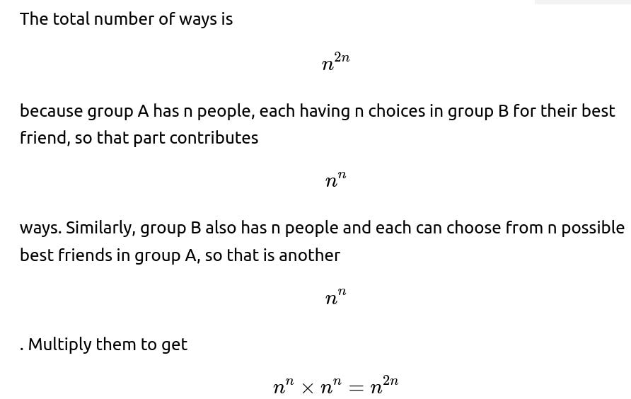
One way to understand this scenario is to think of each group as having exactly n individuals, with every individual in A choosing exactly one “best friend” in B, and every individual in B choosing exactly one “best friend” in A. The total number of ways these choices can be made is n^n for group A (because each of the n users picks from n possible best friends in B) multiplied by n^n for group B, yielding n^(2n) total possible ways of choosing best friends.
A mutual best friendship between a user i in A and a user j in B happens if i chooses j and j also chooses i. The question is about the probability that there are no such mutual pairs at all.
Reasoning with Inclusion-Exclusion
A natural way to tackle this is through the principle of Inclusion-Exclusion:
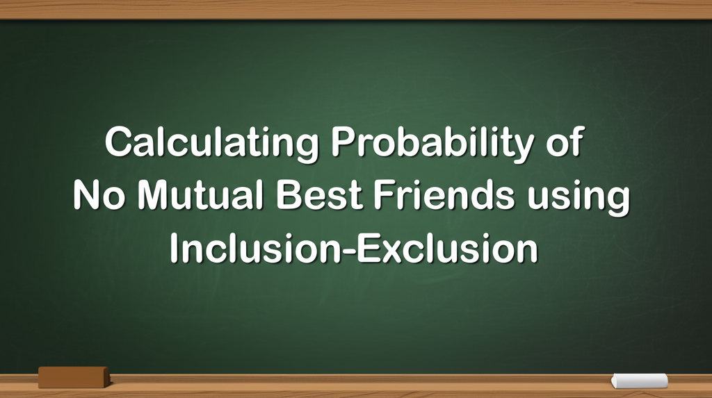
Consider the event that at least one pair (i, j) is a mutual best friend. We want to exclude all such events from the total. The probability of having no mutual best friendships is therefore
Below is the main idea (in an explanatory but concise form, avoiding a full step-by-step chain-of-thought):
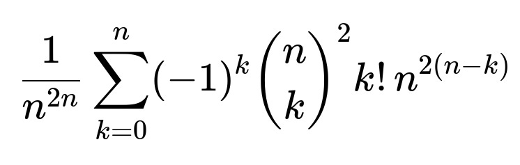
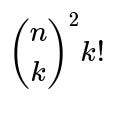
Each term in the Inclusion-Exclusion summation accounts for the possibility that exactly k distinct mutual pairs occur, then alternately adds and subtracts these counts so that we only keep the count of ways with zero mutual pairs. The factor
appears because:
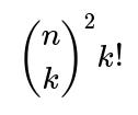
You must choose which k individuals from the A side will be part of these mutual pairs (that gives
ways), and which k individuals from the B side will be involved (another

ways). Then, you need to match these k chosen users on side A with those k chosen users on side B in a one-to-one way, yielding k! possible bijections. Once those k mutual pairs are “locked in,” each of those pairs has no further freedom in its best-friend choice (they must choose each other), so the remaining n – k users in A and the remaining n – k users in B can choose any best friend among n possible users on the opposite side. That contributes
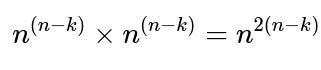
ways for all other users’ choices.
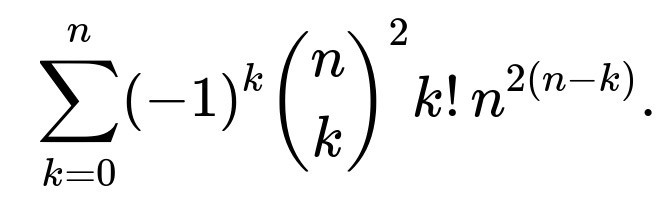
By summing these contributions with alternating signs
ways for all other users’ choices.
By summing these contributions with alternating signs

(which is the hallmark of the Inclusion-Exclusion principle), we count exactly the number of ways to have zero mutual best-friend pairs. Dividing by the total number of ways

converts this count into a probability.
Insights about Large n
When n is large, the expected number of mutual best-friend pairs is close to 1 (because there are n^2 possible cross pairs, each pair has probability 1/n * 1/n = 1/n^2 of being mutual, so the expected count is n^2 * 1/n^2 = 1). This suggests that for large n the number of mutual best friendships behaves approximately like a Poisson(1) random variable, so the probability of having no such pairs is approximately e^(-1).
This aligns with the exact formula tending toward
as n grows large.
Implementation in Python
Here is a short Python snippet that computes this probability exactly for a given n:
def probability_no_mutual_best_friends(n):
    import math

    # total ways
    total_ways = n**(2*n)

    # inclusion-exclusion sum
    sum_no_mutual = 0
    for k in range(n+1):
        # Choose k individuals in A, k in B, match them in k! ways
        choose_pairs = math.comb(n, k) * math.comb(n, k) * math.factorial(k)
        # ways for the rest (n-k in A and n-k in B) to pick best friends freely
        remainder_ways = (n**(n-k)) * (n**(n-k))
        # add or subtract from sum
        sum_no_mutual += ((-1)**k) * choose_pairs * remainder_ways

    # probability
    return sum_no_mutual / total_ways

# Example usage
if __name__ == "__main__":
    for test_n in [1, 2, 3, 5, 10]:
        prob = probability_no_mutual_best_friends(test_n)
        print(f"For n={test_n}, probability of no mutual best friendships = {prob}")
This function uses the exact formula. Note that for very large n, the computation may become expensive or overflow in naive implementations, so special care (such as using logarithms or approximations) might be necessary for extremely large n.
Potential Follow-up Questions Appear Below
What is the total number of ways the best-friend choices can be made, and why?
A subtlety to watch out for is confusing the scenario with a bipartite matching problem. Here, there are no restrictions that must force distinct individuals in B to be chosen by distinct individuals in A (or vice versa). Each user independently picks any one person from the other group.
How do we arrive at the Inclusion-Exclusion formula?
We define “bad” events X_(i,j) = “The pair (i in A, j in B) is mutual best friends.” We want the probability that none of these bad events happen. The Inclusion-Exclusion principle states:
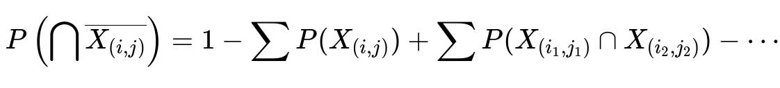
where the sums go over all distinct pairs (i,j). Because a user can only choose exactly one best friend, for multiple mutual pairs to occur simultaneously, they must involve different users on each side, which motivates the factor
when exactly k distinct mutual pairs are forced to occur.
Why is the factor
used for choosing k mutual pairs?
To have k disjoint mutual pairs, you must select exactly k distinct individuals on side A and k distinct individuals on side B. That’s
ways for choosing the subset of A and
ways for choosing the subset of B. After selecting these subsets, you must choose exactly how those k people from A pair up (mutually) with those k people from B. Since each of the k people on A’s side must pair uniquely with one person on B’s side, there are k! ways to permute and match them up.
Could more than one mutual best-friend pair involve the same individual?
No. If user i in A is best friends with user j in B (i chooses j), and that relationship is mutual, then j in B must also have chosen i in A. This means i cannot also be in a second mutual best-friend pair with someone else in B, because each user can choose exactly one best friend. Similarly, j cannot be in a separate mutual pair with a different user from A. Hence, all mutual pairs are disjoint pairs of users.
Can you provide an intuitive understanding of the limit e^(-1)?
When n is large, the number of possible cross pairs (i,j) is n^2, but each has probability 1/n * 1/n = 1/n^2 of being mutual. By linearity of expectation, the expected number of mutual pairs is about 1. In many large random structures where events have small probability but large number, a Poisson approximation is often valid. A Poisson(1) distribution has probability e^(-1) of having zero occurrences. This gives an intuitive reason why the no-mutual probability approaches e^(-1).
How might this problem appear in real-world scenarios?
Even though this is a puzzle-type question, it can apply to analyzing reciprocal relationships in social networks. It’s akin to studying random directed edges (A picks B, B picks A) in a bipartite setting. Understanding the likelihood of mutual connections (or the absence of them) can shed light on random-graph phenomena and help interpret large-scale data from social networks where “favorites” or “best-friend” style choices occur.
What if we wanted to simulate this probability instead of computing it exactly?
One could simulate the process as follows:
You fix n and run many trials. In each trial, have each of the n users in A pick a random user in B, and each of the n users in B pick a random user in A. Count how many mutual picks occur. Record whether the count is zero. Then compute the empirical probability as the fraction of trials that yielded zero mutual pairs. With enough trials, one will approximate the true probability. This is useful if n is large enough that direct computation with factorials and large powers becomes numerically challenging.
Below is a short Python sketch for such a simulation:
import random

def simulate_no_mutual_best_friends(n, trials=10_000):
    count_zero_mutual = 0
    for _ in range(trials):
        # Each user in A picks a friend in B
        picks_A = [random.randrange(n) for _ in range(n)]
        # Each user in B picks a friend in A
        picks_B = [random.randrange(n) for _ in range(n)]

        # Check how many mutual pairs
        mutual_count = 0
        for i in range(n):
            j = picks_A[i]     # A's best friend
            if picks_B[j] == i:
                mutual_count += 1

        if mutual_count == 0:
            count_zero_mutual += 1

    return count_zero_mutual / trials

# Example usage
if __name__ == "__main__":
    estimated_prob = simulate_no_mutual_best_friends(5, 100000)
    print(f"Estimated probability (n=5) with 100k trials: {estimated_prob}")
This brute-force simulation, of course, becomes slower for large n, but it may still be practical for moderate n.
What are key pitfalls in implementing the exact or approximate solutions?
One potential pitfall is integer overflow or floating-point underflow if n is large and the computation of n^(2n) or factorial(k) becomes huge. One typically remedies this by performing careful logarithmic arithmetic or by relying on approximations (e.g., using e^(-1) for large n).
Another pitfall is to accidentally allow an individual on one side to choose multiple best friends or to count pairings incorrectly. It is important to remember that each user picks exactly one best friend, so each user’s choice is exactly one edge, and these edges are directed (A to B, B to A). That uniqueness drives the combinatorial factors in the Inclusion-Exclusion formula.
How might you explain the Inclusion-Exclusion approach to a colleague new to advanced combinatorics?
You might say: “Think of each potential mutual pair as an event we want to avoid. If you try to count how many ways you can avoid all of them, you can start by subtracting off the ways that any one event happens, then add back the ways that any two events happen (because you subtracted them twice), subtract the ways that three events happen, and so on. Since each pair of events can only happen simultaneously if they don’t share individuals, that’s where we multiply by
for choosing which k pairs occur.”
Below are additional follow-up questions
Could we approach the problem using a Markov chain perspective?
Yes, one can theoretically conceive of a Markov chain whose states encode how many mutual best-friend pairs currently exist (or more detailed microstates capturing which specific pairs are mutual). However, building such a chain explicitly can be cumbersome.
A potential Markov chain approach might go like this:
You consider all possible ways that the n users in A and the n users in B can choose best friends. This set of configurations can be seen as the state space of the chain. Since each side has n users and each user picks exactly one among n options, there are (n^{2n}) total states.
You would then define a transition rule, for example, a single user in A or B randomly switches their choice to a new best friend at each step. Over time, the chain would explore the configurations.
If your goal is to estimate the probability of zero mutual best-friend pairs, you could theoretically let the chain run long enough, reach a stationary distribution, and measure how often it’s in a state of zero mutual pairs. Because this problem is uniform—each configuration is equally likely—if the Markov chain is ergodic and covers all states equally in the stationary distribution, the chain would converge to the uniform distribution over states. Then the fraction of time spent in states with zero mutual friendships would converge to the same probability given by the Inclusion-Exclusion formula.
Pitfalls and subtleties:
The Markov chain must be carefully designed to be aperiodic, irreducible, and to have the uniform distribution as its stationary distribution.
The state space is very large ((n^{2n})). Even for moderate n, enumerating or effectively mixing in that space can be challenging.
Convergence times might be prohibitive, especially if n grows. In practice, you would rely on approximate methods or specialized sampling to ensure good coverage.
Real-world analogy:
If each user’s best friend choice might spontaneously change to a new person, then analyzing the system as a Markov chain might illuminate the long-term fraction of mutual best-friend states. But one must ensure the chain is well-mixed.
How can we estimate or calculate the distribution (not just the probability of zero) of the number of mutual pairs?
We can go beyond just the probability of zero mutual best-friend pairs and look at the entire distribution of how many mutual pairs exist. Some points:
Expected Value By linearity of expectation, the expected number of mutual best friends is 1 for any n. Specifically, each of the (n^2) cross pairs has probability (1/n \times 1/n = 1/n^2) of being mutual, so expectation is (n^2 \times (1/n^2) = 1).
Variance and Higher Moments To get the variance, you need to account for correlations among different pairs. A pair (i, j) being mutual can affect whether (i, k) or (k, j) can also be mutual because i or j might already have used their one choice.
Exact Distribution
You can try to extend the Inclusion-Exclusion principle to handle the probability that exactly k pairs are mutual. This is similar to the combinatorial expression for zero pairs but arranged to count precisely k pairs.
The probability of having k mutual pairs involves selecting those k pairs in a disjoint way, then letting the remaining choose freely.
Poisson Approximation For large n, the number of mutual pairs is approximately (\text{Poisson}(1)). Under that approximation, the probability of exactly k mutual pairs is about (\frac{e^{-1}}{k!}). Thus, the distribution is heavily centered around 0, 1, 2, … with a mean of 1. For large n, the probability of no mutual pairs is about (e^{-1}), exactly matching the k=0 term in the Poisson(1) distribution.
Potential pitfalls:
Directly computing the entire distribution via naive combinatorial sums can be expensive if you try to handle large n.
Approximations (Poisson, or possibly even normal approximations) might be used incorrectly if n is small. For smaller n, you’d want the exact method or a direct enumeration or simulation to get the distribution.
What if some individuals in A or B have a preference distribution rather than choosing uniformly at random?
If, instead of each user choosing a best friend uniformly, they choose according to some probability distribution (like user i in A has probabilities (p_{i,1}, p_{i,2}, \ldots, p_{i,n}) over B), the problem changes:
Each cross pair (i in A, j in B) now has probability (p_{i,j} \times q_{j,i}) of being mutual, where (q_{j,i}) is B’s probability distribution for user j choosing user i.
The expected number of mutual pairs is (\sum_{i=1}^n \sum_{j=1}^n p_{i,j} q_{j,i}).
The probability of zero mutual pairs must again rely on a generalized Inclusion-Exclusion, but the uniform simplifications become more complicated because each pair might have different probabilities. This can lead to more involved combinatorial sums.
Edge cases:
Some (p_{i,j}) might be zero for certain j, meaning user i absolutely does not pick j. This eliminates certain events in the Inclusion-Exclusion sum and can drastically alter the probability.
If preferences are heavily skewed (e.g., every user in A picks only the same single user in B with probability close to 1), you can easily get a high chance of a mutual pair or see interesting degenerate cases.
Real-world usage:
In many social platforms, user preferences are not always uniform. Some users might be extremely popular, so many in A choose them. The chance of reciprocal “best friend” might be different from the uniform assumption. Analyzing the system with custom preference probabilities can reveal more accurate real-world predictions.
How does this analysis extend if each user can choose more than one best friend?
A different variant is: each user in A picks exactly d distinct best friends from B, and each user in B also picks exactly d distinct best friends from A, with all choices random among the n possible candidates. A mutual best-friend pair means that user i in A has user j in B in their set of d best friends, and user j in B also includes user i in their set of d best friends.
Key changes:
The total number of ways for each side is (\binom{n}{d}^n) if each user picks d distinct best friends from n choices. (This is because each of the n users chooses a combination of size d from n possible.)
The chance that a specific (i, j) is in each other’s chosen set is ((d/n) \times (d/n)) if the choice is uniform among all (\binom{n}{d}) subsets, though the exact calculation needs careful thought because we have combinatorial constraints rather than purely independent picks.
The expected number of mutual pairs is then (n^2 \times \Pr(\text{mutual})). But (\Pr(\text{mutual})) depends on how the subsets are chosen. In a purely combinatorial sense, user i in A includes j in B with probability (d/n), and user j in B includes i in A with probability (d/n), so one might guess (\Pr(\text{mutual}) \approx (d/n)^2). But the picks are not necessarily independent across different individuals. Careful or approximate arguments could be used.
Pitfalls:
If d is large relative to n, it increases the chance of mutual pairs. If d = n, everything is trivially mutual. If d = 1, we revert to the original scenario.
Inclusion-Exclusion becomes more involved. Counting ways where exactly k pairs are mutual might get significantly more complicated because multiple pairs can overlap in terms of the same user if they have capacity to choose multiple best friends.
Practical scenario:
This might arise if, say, on a platform each user can mark up to d “favorite” or “best” contacts. The question “What is the probability no two people mutually rank each other?” can become relevant in certain viral marketing or recommendation contexts.
Can we connect this to the concept of derangements, and is that helpful?
Derangements are permutations on a single set where no element maps to itself. A classical example: “How many ways can you seat n people so that nobody sits in their own seat?” In that problem, for each i, i can’t map to itself. This yields a known formula with a well-known limit (1/e).
Here, the best-friend scenario superficially feels “like a derangement problem,” but it is not exactly the same. The reason:
In a derangement, we have a single set of size n and a permutation function from that set to itself with the restriction that f(i) ≠ i.
In the mutual best-friend problem, we have two distinct sets A and B, each with n members, and each user picks exactly one best friend from the other group. “Mutual” corresponds to a 2-cycle in the bipartite directed graph, not a 1-cycle (fixed point) in a permutation.
Nonetheless:
The probability that no user “chooses themselves” in a derangement scenario is the fraction of derangements among all permutations, which is about 1/e for large n.
The probability that no pair chooses each other in our problem similarly tends to e⁻¹.
Both results revolve around an exponential boundary, but the details are different. The bipartite nature changes the combinatorial counting.
Pitfalls:
Over-applying the concept of derangements could lead to confusion if one tries to map the bipartite scenario incorrectly to a standard single-set permutation problem. You’d need a perfect matching or permutation from A to B and from B to A, which is not the same as each user picking exactly one out of n choices with no global constraint about distinctness.
How can we handle the case when n is extremely large, from a computational standpoint?
For extremely large n, directly using the exact formula involving factorials and powers is impractical because:
(n^{2n}) can be astronomically large. Even storing that number is impossible for large n.
The sum in the Inclusion-Exclusion formula requires computing big binomial coefficients (\binom{n}{k}) and factorials up to k!.
Practical solutions:
Poisson Approximation For large n, we can rely on the argument that the expected number of mutual pairs is about 1 and that the distribution is approximately Poisson(1). Thus, the probability of zero mutual pairs is about (e^{-1}).
Simulation You can run large-scale simulations if n is not too huge (e.g., a few thousands or tens of thousands). Each simulation involves generating random best-friend choices for A and B, checking how many mutual pairs result, and averaging over many trials.
Stochastic / Monte Carlo To get a very precise estimate, a Monte Carlo approach can be used. Instead of enumerating all possibilities, we sample a large number of random configurations and measure the fraction that yields zero mutual best friends.
Pitfalls:
For extremely large n (like millions), even a single simulation might be big. However, simulating is often more tractable than enumerating all possibilities or summing enormous combinatorial terms.
The Poisson approximation’s accuracy might be questioned for certain edge cases. If the random choices are not i.i.d. or if n is large but the selection is not uniform, the e⁻¹ approximation might deviate.
Memory constraints can appear if you try to store each user’s choice in an array of size n for A and n for B at extremely large scale. You might need a streaming approach or do partial sums.
If the set sizes differ (say, |A|=m and |B|=n with m ≠ n), how does it change the probability?
In that scenario, each user in A picks from the n members of B, and each user in B picks from the m members of A. The total ways to choose:
A side: (n^m) ways, since each of the m users in A chooses from n in B.
B side: (m^n) ways, since each of the n users in B chooses from m in A.
Overall total ways: (n^m \times m^n).
A pair (i in A, j in B) is mutual if i chooses j and j chooses i. The analysis is somewhat more involved:
There are m × n possible cross pairs.
Each pair’s probability of being mutual is (\frac{1}{n} \times \frac{1}{m} = \frac{1}{mn}), if everything is uniform.
The expected number of mutual pairs is m × n × (1/(mn)) = 1, so interestingly that part is still 1.
The probability of no mutual pairs can be handled by an Inclusion-Exclusion approach again, but the combinatorial formula modifies to:
Choose k pairs out of the possible min(m, n) that can be formed in a disjoint way. That requires selecting k individuals out of m from A, k individuals out of n from B, and k! permutations.
Each forced mutual pair restricts those users from forming any other mutual pair.
The remaining (m-k) from A have n choices each, and the remaining (n-k) from B have m choices each, so that part yields (n^{(m-k)} \times m^{(n-k)}).
Hence the sum for exactly k forced mutual pairs has a factor (\binom{m}{k} \binom{n}{k} k! n^{(m-k)} m^{(n-k)}) with alternating signs. Dividing by (n^m m^n) yields the probability. As n and m grow large but keep some ratio (\alpha = m/n), you might still get an approximate Poisson(1) argument, leading to a probability near e⁻¹ for zero mutual pairs, although subtle difference can arise if (\alpha) is extremely large or small.
Pitfalls:
If m ≠ n, the combinatorial formula and any direct code must reflect the asymmetry.
If one group is much larger than the other (e.g., m >> n), the probability of mutual pairs might be higher or lower depending on how the random choices concentrate.
The intuitive approximate argument that the expected number of pairs is 1 still often leads to a Poisson(1)–like approximation for large m, n, but the ratio can influence the distribution’s shape in smaller-scale cases.
How does random variation in group size or user participation affect the result?
Consider real-world scenarios where not exactly n but “about n” people in each group are active or some fraction are offline:
If the active group sizes fluctuate, you might get a distribution of group sizes. For each realized size, the probability of zero mutual pairs might differ slightly. You would effectively have to take an expectation over the distribution of group sizes as well.
In practical platform analytics, user activity might be unpredictable, so you might measure an average probability of zero reciprocal relationships by convolving the formula over possible user counts.
Pitfalls:
Must be careful that the random group sizes don’t break the assumption that each user picks exactly one best friend from the entire group. If the group is dynamic, or a user is offline, that user might not make a choice at all.
If the group size changes drastically, the approximation e⁻¹ might no longer be stable.
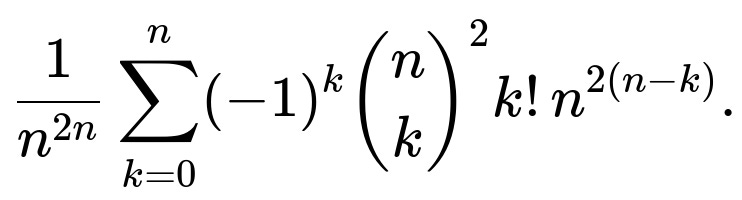
Are there combinatorial or algebraic simplifications to the Inclusion-Exclusion sum that might yield a closed form?
The known closed form for the original scenario (two groups each of size n) is:
It does not collapse to a simpler elementary expression for arbitrary n. One might rewrite it or factor out common terms, but typically there is no “simpler” expression in elementary functions.
You can do some rewriting:
Factor out (n^{2n}) to see the probability explicitly as:
You can factor out (n^{2(n-k)}) in each term:
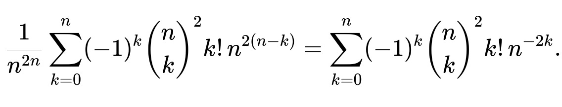
That last summation is possibly more stable numerically for large n because you’re dividing by (n^{2k}) in each term. However, it still is a finite sum of length (n+1), so no simpler closed form in basic functions is known.
Pitfalls:
Attempting to simplify further may lead you in circles or toward special functions not typically covered in basic algebraic manipulations.
For large n, using that summation directly is still large in intermediate steps (binomial coefficients can be huge), so you would do a log-based approach or rely on the e⁻¹ approximation.
Could partial or incomplete reciprocity be relevant, like measuring the fraction of users in A who are chosen back by their picks in B?
Yes. One could also be interested in partial measures, for example: “Among the n users in A, how many are ‘reciprocated’ by the user they picked in B?” That is effectively the distribution of how many people in A have a mutual relationship. Similarly, from B’s perspective, how many people in B get chosen back by the user they picked in A?
Such questions revolve around the distribution of the random variable “number of mutual best friendships from one side’s point of view.” That variable might be correlated with the total number of mutual best friendships but is not identical. One approach is:
Let X = number of users in A who form a mutual best friendship with whomever they picked in B.
Then X is the count of i in A such that if i picks j in B, user j in B picks i back.
The expected value of X is still 1 if we consider all pairs, but now we have a sum of n indicator random variables, each for a user i. Each user i in A has probability 1/n of picking j, and that j in B has probability 1/n of picking i, so the probability that i is in a mutual relationship is 1/n.
Pitfalls:
The distribution of X might be slightly different from the total count of mutual pairs in the entire system because from B’s perspective, some other set of pairs might be mutual.
The sum of “how many in A are in mutual pairs” and “how many in B are in mutual pairs” must be the same total, but the random variable from each side’s perspective can have interesting conditional properties.
Could knowledge of this problem help in designing or analyzing recommendation engines, especially for “mutual” preferences or matches?
In a broad sense, yes:
Recommendation engines often try to predict user-to-user or user-to-item “matches.” In bipartite item-user settings, a “mutual best friend” might correspond to a scenario where the user picks an item, and the item is specifically recommended for that user—akin to a personalized content curation.
In user-user recommendation (like dating apps or friend suggestions), “mutual likes” or “mutual swipes” can be seen as edges in a bipartite or single-graph setting. Understanding the probability of no mutual matches can help set expectations on how many stable matches or mutual acceptances you might get from random behavior.
Subtlety and pitfalls:
In real systems, user behavior is far from uniform. People have preferences, biases, or rely on recommendation algorithms that shape their choices.
The random uniform model is useful as a baseline or “null model,” but actual data typically deviate.
If designers want to ensure a certain fraction of mutual matches, they might implement algorithms that nudge or facilitate more reciprocation. This problem’s analysis clarifies how the random baseline can lead to about e⁻¹ chance of no matches (or 37%) if the user sets are equal in size. Real algorithms often aim to reduce that “no-match scenario” significantly.
How does one verify the correctness of the formula through small n test cases?
A common approach is to do an exact enumeration for small n:
n=1
Group A has 1 person (call them A1), Group B has 1 person (B1).
A1 picks B1 with probability 1, B1 picks A1 with probability 1, so there is always a mutual best friendship. Probability of zero mutual is 0.
The formula for zero mutual pairs:
(\binom{1}{0}^2 0! , 1^{2(1-0)} (-1)^0 + \binom{1}{1}^2 1! , 1^{2(1-1)} (-1)^1 = 1 + (-1)\times 1^2 \times 1 = 1 - 1 = 0.)
Matches the direct analysis.
n=2
We can systematically list out the possibilities: 2 choices for A1 (which of B1 or B2 to pick), 2 choices for A2, 2 choices for B1, 2 choices for B2, for a total of (2^4 = 16) possible configurations. Count how many have zero mutual pairs. Then compare to the formula.
Formula approach:
Total ways: (2^4 = 16.)
For zero pairs, Inclusion-Exclusion sum:
k=0 term: (\binom{2}{0}^2 , 0! , 2^{2(2-0)} = 1 \times 1 \times 2^4 = 16.)
k=1 term: (\binom{2}{1}^2 , 1! , 2^{2(2-1)} (-1)^1 = (2 \times 2) \times 1 \times 2^2 \times (-1) = 4 \times 4 \times (-1) = -16.)
k=2 term: (\binom{2}{2}^2 , 2! , 2^{2(2-2)} (-1)^2 = (1 \times 1) \times 2 \times 2^0 \times 1 = 2.)
Sum = 16 - 16 + 2 = 2. Probability = 2/16 = 1/8.
One can confirm by direct enumeration or simulation. So the formula checks out.
Pitfalls:
Implementing enumeration incorrectly (e.g., forgetting that each user can pick the same friend or missing some configuration) can lead to mismatch with the formula.
If a developer tried to implement the formula but used the wrong sign or misapplied combinatorial terms, they might get an incorrect result that fails to match small-n enumerations.
If we allow for the possibility that a user might not choose anyone (or might choose “no best friend”), how does that affect the analysis?
In that variant, each user has n+1 “choices”: the n possible users of the other group plus an option “none.” Then:
The total ways are ((n+1)^n \times (n+1)^n = (n+1)^{2n}) if both sides have n users.
A pair is mutual only if both pick each other, meaning neither chooses “none.”
Inclusion-Exclusion becomes more intricate, because for a pair (i, j) to be forced mutual, i picks j out of n+1, j picks i out of n+1, and you also have to consider the possibility that some other user picks “none.”
Pitfalls:
Not everyone necessarily chooses a real friend, so you can’t just do the simpler n^n approach.
If you don’t treat the “none” choice carefully, you might miscount or incorrectly compute probabilities of events.
For large n, a fraction of people might pick “none,” changing the expected number of mutual pairs.
Use cases:
In real systems, a user might not specify a best friend if they are inactive or if the feature is optional. The probability of zero reciprocal pairs might go up since “none” becomes an easy choice.
Does the problem’s logic hold if we interpret “best friend” as a preference ranking with a single top choice?
Yes. The central assumption is that each user makes exactly one top pick. That single top pick, if reciprocated, yields a mutual pair. The mathematics rely on each user making exactly one choice out of n possibilities. Any scenario that adheres to that structure—like “choose your absolute favorite out of n possible friends”—follows the same logic.
Potential confusion arises if:
You allow partial ranking or multiple top choices. Then the combinatorial counts differ.
A user can be forced to rank all possible friends in some order, but only the top is what matters for the “best friend” link. In that case, we effectively ignore the rest of the ranking and just focus on the top selection for each user.
Edge cases:
If the “best friend” must come from a subset or if there is some mechanism that not everyone can pick the same user, the uniform assumption breaks.
If multiple users in A cannot pick the same user in B, that changes the problem entirely. Then you have constraints akin to perfect matchings in bipartite graphs, not purely random independent picks. The probability of zero mutual pairs will be different.
How would you test a candidate in a FANG interview to ensure they fully understand this problem?
Some potential angles for an interviewer:
Combinatorial reasoning
Ask the candidate to articulate how many total ways of choosing best friends exist and why it’s (n^{2n}).
See if they can reason about why the probability of no mutual pairs might converge to (e^{-1}).
Implementation details
Have them write code to compute or approximate for small n.
Ask them about how they’d handle large n.
Edge cases
Ask how the formula changes if n = 1 or n = 2, or if the groups have unequal sizes.
Ask what if each side must choose distinct best friends (i.e., a matching constraint).
Connection to known distributions
Ask them to relate the result to the Poisson approximation or to derangements and highlight the similarities and differences.
Real-world data scenario
Present a scenario in a large social network with non-uniform user picking and see if they can adapt the reasoning or discuss how to approximate.
Pitfalls to watch for in the candidate’s understanding:
Confusing the bipartite random picking with permutations on a single set.
Failing to see the link between expected number of pairs and the Poisson approximation for large n.
Not recognizing the factorial and binomial terms in the Inclusion-Exclusion sum.
How can one ensure numerical stability if implementing the formula for moderately large n (like n=30 or n=50)?
When n is around 30 or 50:
Direct factorial or large power calculations might exceed normal integer ranges unless you use a language or library that supports big integers (e.g., Python’s arbitrary precision integers).
Floating-point computations might lose precision if done naively. So a typical approach is to work in logarithms. For example:
Compute (\log(\binom{n}{k})) using a precomputed factorial log table or a function that sums (\log(i)).
Accumulate sums in log space.
Finally exponentiate at the end. Or, if you only need the ratio to (n^{2n}), you can keep track of (\log(\text{numerator}) - \log(\text{denominator})).
Pitfalls:
Rounding errors can accumulate if you do many additions or subtractions of logs.
If you do alternating sums in linear space, huge cancellations could cause a catastrophic loss of precision.
Using an extended precision library or carefully structuring the sum from smallest terms to largest might help.
What if the friendship or best-friend choice is not strictly bipartite, i.e., everyone is in one big group and each person picks one best friend among the entire set (excluding themselves perhaps)?
That scenario becomes a random directed graph on n nodes where each node chooses exactly one outgoing edge to another node (possibly excluding themselves). Now a “mutual best friendship” is a 2-cycle in that directed graph. The total ways each node can choose a friend is ((n-1)^n) if we exclude self-friendship. Counting the probability of no 2-cycle is akin to counting the fraction of directed graphs with outdegree exactly 1 that have no 2-cycle.
The approach:
We could again use Inclusion-Exclusion, but the combinatorial factors differ. Instead of picking from two sets, we pick from the same set with no repetition of identity. If i picks j, that means an edge from i to j. For a 2-cycle to form, j picks i as well. The counting pattern is more reminiscent of the concept of “functional digraphs” (since each node has exactly one outgoing edge, the graph is a union of directed cycles and directed trees merging into those cycles).
Pitfalls:
The bipartite logic with n^n × n^n does not apply. Instead, we have ((n-1)^n) total ways if self-friendship is disallowed, or (n^n) if self is allowed.
The probability of no 2-cycle in a random “functional digraph” can still lead to a Poisson(1/2) or similar limit, depending on the constraints. The exact distribution might approach e^(-c) for some constant c. But it’s a different constant from bipartite picking.
Real-world difference:
On many social platforms, you do only pick from the opposite set (like a teacher picks a student in a school setting or a single picks a prospective partner from a pool) versus picking from the entire population. The difference is crucial to the combinatorial structure.
What if each user in A picks a best friend in B with probability proportional to some weighting, and similarly from B to A, but the weights are not uniform?
This is a generalization of the “preference distribution” scenario. Suppose user i in A has a preference vector ((w_{i,1}, w_{i,2}, \dots, w_{i,n})), and user i picks j with probability proportional to (w_{i,j}). Similarly, each user j in B picks i in A with probability proportional to some other weighting. Then:
The probability that (i, j) is a mutual best friendship is (\frac{w_{i,j}}{\sum_{k=1}^n w_{i,k}} \times \frac{v_{j,i}}{\sum_{\ell=1}^n v_{j,\ell}}), if we denote B’s preference as (v_{j,i}).
The probability of zero mutual pairs is more complicated because you have to incorporate the fact that each user only picks exactly one friend (but from a distribution, not uniform). You can still do an Inclusion-Exclusion approach, but each event “(i, j) is mutual” now has a different probability, and subsets of events have to be carefully combined.
Practical significance:
Recommendation systems often have non-uniform weights, e.g., a user is more likely to pick close geographic neighbors or those with certain attributes.
The formula is no longer symmetrical or purely in closed form. Typically, you’d do an approximate or simulation approach.
Pitfalls:
If you assume independence incorrectly, you might incorrectly multiply probabilities for overlapping events that share an individual. The single-choice constraint breaks naive factorization.
Real preference data can be sparse (some weights might be zero or extremely large), so you must handle corner cases carefully.
Could knowledge of generating functions help approach or check this result?
Generating functions can be used sometimes to manage the counting of objects with constraints, but the direct Inclusion-Exclusion approach is usually more straightforward here. One might:
Try to form an exponential generating function or ordinary generating function for the ways that k mutual pairs occur.
Identify a combinatorial class (like sets of 2-cycles plus directed edges) and use combinatorial species theory.
However, the result typically loops back to something akin to the same sum we’ve written. So while generating functions might be interesting academically, they don’t necessarily simplify the final probability expression for no mutual best friendships.
Pitfalls:
Constructing a generating function might be complicated because each user’s choice depends on exactly one pick, and we have a bipartite system.
The partial results for large n might just reaffirm the e⁻¹ approximation.
Is the probability of no mutual pairs monotonic in n?
It actually decreases as n grows. When n=1, the probability of no mutual best friendship is 0. For n=2, we found 1/8. For n=3, it’s bigger than 1/8 but less than e⁻¹, typically. Then as n → ∞, it converges to e⁻¹ ≈ 0.3679..., which is larger than 1/8 = 0.125. This indicates the probability of having zero mutual friends actually rises from small n to some region, then eventually stabilizes around e⁻¹. The sequence is not strictly monotonic from n=1 to n=∞ in the sense of always going up or always going down—there might be some crossing points.
Pitfalls:
If one incorrectly assumes it always increases or always decreases, they might be surprised by actual numerical values at small n. Checking small n explicitly is instructive.
The limit is e⁻¹ but for n=2 it is 1/8 which is 0.125, whereas e⁻¹ is about 0.3679. So the probability jumps up somewhere between n=2 and n=∞.
Could the concept of adjacency matrices help clarify the scenario?
We might represent the bipartite picks as a pair of adjacency matrices:
(A_{ij} = 1) if user i in A picks user j in B, else 0. Each row i in A’s adjacency matrix has exactly one “1.”
(B_{ji} = 1) if user j in B picks user i in A, else 0. Each row j in B’s adjacency matrix has exactly one “1.”
A mutual best friendship between i and j implies (A_{ij} = B_{ji} = 1.)
One could try to reason about the matrix product (A \times B) or similar constructs, but each matrix is not square in the same dimension (A is n×n for picks from A to B, B is n×n for picks from B to A, but from B’s perspective, the adjacency might be transposed if you use consistent indexing). The main significance is just to see that each row has exactly one “1.” We are basically looking for positions (i, j) that are symmetrical.
Pitfalls:
People might incorrectly think of i picking j as a standard adjacency in a single matrix with i, j in the same set. Actually, we have two sets, so the adjacency structure is bipartite.
The matrix perspective is more helpful if we want to do linear algebra or network analysis. But for the probability of zero mutual edges, the combinatorial argument remains more direct.
Are there any known applications where the probability of no mutual best friendships must be minimized or maximized?
In matching-based or pairing-based systems, sometimes you want to avoid zero mutual matches (like in dating apps or friend recommendation systems). You might want to design the system so that the chance that no pairs match is extremely low. If we rely purely on random user choices, the chance might be around e⁻¹ for large n. If that’s undesirable, the platform might incorporate:
Weighted suggestions or constraints to push reciprocation.
An algorithm that ensures that if a user in A picks user j in B, B might get a “hint” that A picked them and become more likely to pick them back.
In contrast, in certain load-balancing or resource-allocation problems, having no mutual “overlap” might be beneficial. For instance, if “mutual best friendship” indicates a conflicting assignment, the system might want to reduce or eliminate it.
Pitfalls:
Over-engineering the system to guarantee mutual pairs might inadvertently cause heavy biases or be gameable by users.
Minimizing or maximizing the fraction of mutual picks depends heavily on a platform’s objective, which may conflict with user autonomy or natural usage patterns.
If we want to confirm the Poisson approximation more rigorously for large n, how might we proceed?
A more formal argument typically involves:
Defining indicator random variables (X_{ij}) = 1 if (i in A, j in B) form a mutual pair, else 0. Then the total number of mutual pairs is (X = \sum_{i=1}^n \sum_{j=1}^n X_{ij}.)
Showing that (X_{ij}) are approximately independent for large n, in the sense that the covariance among different pairs is small compared to the total. Indeed, if (i, j) is mutual, it forces i and j not to be mutual with anyone else, but for large n, this effect is relatively minor overall.
Applying a classical limiting theorem for sums of many weakly dependent Bernoulli variables with small means, leading to a Poisson(λ) limit with λ = E[X] = 1.
Pitfalls:
Overlapping dependencies can complicate a naive independence assumption, but advanced theorems (like the Chen-Stein method for Poisson approximation) handle these dependencies.
For smaller n, the exact distribution can deviate from Poisson; the approximation becomes better with increasing n.