
ML Interview Q Series: Calculating Win Probability for a Two-Game Lead Match Using Conditional Probability.

Browse all the Probability Interview Questions here.
Bill and Mark play a series of games until one of the players has won two games more than the other player. Any game is won by Bill with probability p and by Mark with probability q = 1 - p. The results of the games are independent of each other. What is the probability that Bill will be the winner of the match?
Short Compact solution
Define A as the event that Bill wins the match. Using conditional probability on the events that Bill loses 0, 1, or 2 of the first two games, we can write:
A direct computation shows: A) If Bill loses 0 of the first two games, Bill already has a two-game lead and immediately wins. B) If Bill loses 1 of the first two games, we use the fact that the probability of eventually winning remains P(A). C) If Bill loses both of the first two games, he has already lost the match.
Hence one obtains:
Since p^2 + 2 p q + q^2 = (p + q)^2 = 1, we see that 1 - 2 p q = p^2 + q^2. Equivalently, the gambler's ruin formulation (starting with two “units” for Bill and two for Mark) arrives at the same probability:

Comprehensive Explanation
Overview
We want the probability that Bill becomes exactly two games ahead of Mark at some point in an indefinite sequence of independent Bernoulli(p) trials. Each trial corresponds to a single game, which Bill wins with probability p and Mark wins with probability q = 1 - p.
Core Reasoning via State Transitions
It is often helpful to view this scenario as a Markov chain where the “state” is (Bill’s wins - Mark’s wins). Initially, the state is 0 (because no one is ahead). After each game:
If Bill wins, we move the state by +1.
If Mark wins, we move the state by -1.
The match ends when the state hits +2 (Bill ahead by 2) or -2 (Mark ahead by 2). We want the probability that the state eventually hits +2 rather than -2.
Formal Approach
One direct method uses conditional probabilities based on how the first two games unfold:
Bill loses 0 of the first two games (probability p^2). In that case, Bill is already ahead by 2 games, so Bill wins with probability 1.
Bill loses 1 of the first two games (probability 2 p q). The score difference is 0 again (because Bill won 1 game and Mark won 1 game), and from that situation, the probability of Bill eventually winning is still P(A).
Bill loses 2 of the first two games (probability q^2). In that case, Mark is already ahead by 2 games, so Bill’s probability of winning is 0.
Thus,
P(A) = p^2 * 1 + (2 p q) * P(A) + q^2 * 0.
Solving for P(A):
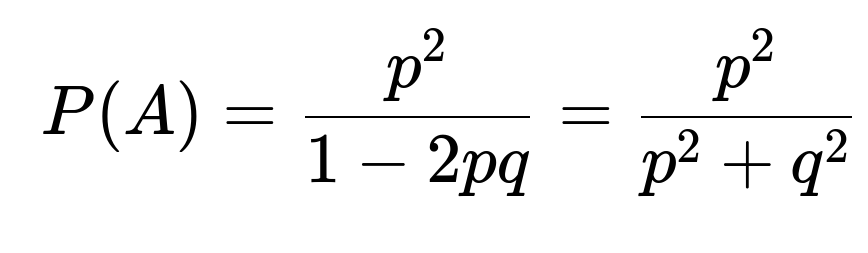
p^2 + 2 p q P(A) = P(A) ⇒ P(A) - 2 p q P(A) = p^2 ⇒ P(A) (1 - 2 p q) = p^2 ⇒ P(A) = p^2 / (1 - 2 p q).
Since p^2 + 2 p q + q^2 = (p + q)^2 = 1, it follows that 1 - 2 p q = p^2 + q^2. Hence,
P(A) = p^2 / (p^2 + q^2).
Alternative Gambler’s Ruin Interpretation
This problem mirrors a gambler’s ruin scenario with “Bill’s net position” determined by how many more games he has won than Mark. Both start at 0 difference, and the absorbing boundaries are at +2 (Bill wins) or -2 (Mark wins). From the standard gambler’s ruin analysis for an unbiased or biased random walk with absorbing states, the same formula emerges:
P(A) = p^2 / (p^2 + q^2).
If p = 0.5, this formula simplifies to p^2 / (p^2 + q^2) = (0.5^2)/(0.5^2 + 0.5^2) = 0.25 / 0.5 = 0.5, which aligns with the intuitive idea that if Bill and Mark have the same skill, Bill’s chance of eventually getting two games ahead is 50%.
Simulation Perspective (Optional Check)
We can numerically verify this probability with a small Python simulation:
import random

def simulate_one_match(p=0.3, num_repetitions=10_000_00):
    # p is probability Bill wins a single game
    # returns fraction of matches that Bill wins
    Bill_wins_count = 0
    for _ in range(num_repetitions):
        diff = 0
        while abs(diff) < 2:
            if random.random() < p:
                diff += 1
            else:
                diff -= 1
        if diff == 2:
            Bill_wins_count += 1
    return Bill_wins_count / num_repetitions

result = simulate_one_match(p=0.3, num_repetitions=1000000)
print("Simulation Probability Bill Wins:", result)
As we increase num_repetitions, the simulation’s fraction should converge to p^2 / (p^2 + q^2).
Follow-up question 1
How does the probability change if p = 0.5?
When p = 0.5, Bill and Mark are equally skilled. Then q = 1 - p = 0.5. In that case:
p^2 = 0.25 and q^2 = 0.25.
Hence p^2 + q^2 = 0.5. So Bill’s probability of eventually getting two games more than Mark is 0.25 / 0.5 = 0.5. This means it is an even 50-50 chance if both have equal probability of winning any given game.
Follow-up question 2
What if p is very close to 1 or very close to 0?
If p is very close to 1, Bill almost always wins each individual game, so p^2 dominates over q^2. Then p^2 / (p^2 + q^2) is close to 1. Conversely, if p is very close to 0, then q^2 is nearly 1, making p^2 / (p^2 + q^2) very small, and Bill has almost no chance of achieving a two-game lead.
Follow-up question 3
Is there an intuitive explanation for the p^2 / (p^2 + q^2) result?
One intuitive explanation is that the event “Bill wins by eventually getting a 2-game lead” is balanced against the symmetric event “Mark eventually gets a 2-game lead.” If Bill’s likelihood of winning each game is p, Mark’s is q. Think of the ratio p^2 : q^2 as a measure of whose “2 consecutive successes” is more likely when the match extends long enough. The factor p^2 + q^2 then quantifies the total “weight” of Bill’s two-game-run possibility and Mark’s two-game-run possibility, ignoring the intermediate back-and-forth states that reset the difference to zero. Bill’s final probability is Bill’s portion of that total.
Below are additional follow-up questions
What if there is a maximum number of games allowed?
In some real-world tournaments, a maximum number of games might be enforced (for instance, if organizers have limited time, they might say there will be at most N games). If neither player is 2 games ahead by the time those N games are played, you might call it a draw or use some other tiebreaker. This imposes an artificial cutoff on the random process.
Key Insight: With a maximum N, the probability that Bill gets 2 games ahead must be modified because there is now a positive probability that the match could end without either player being 2 games ahead. Mathematically, you would need to consider a truncated state-space for the Markov chain: states would go from -2 to +2, but you also stop if you have played N total games.
Pitfall: Analyzing the probability that Bill leads by +2 before time N can be tricky, especially for large N. You must sum over all possible paths that arrive at +2 for the first time on or before game N.
Edge Case: If N < 3, Bill cannot achieve a +2 lead nor can Mark, so the probability Bill is 2 ahead is obviously 0 in such a severely truncated scenario.
How do we compute the expected number of games until one player leads by 2?
While the main question is about the probability of Bill winning, an interviewer might also ask about the expected duration (i.e., the expected number of games). The process is a random walk on {-∞, ..., -1, 0, 1, ..., +∞}, but practically, it stops at +2 or -2.
Approach: One way to find the expected duration is to solve a system of linear equations for the expected time to absorption in a Markov chain, focusing on states {-1, 0, +1}, because -2 and +2 are absorbing. Each state’s expected time can be expressed in terms of the expected time from the next possible states:
E(0) = 1 + p * E(1) + q * E(-1) E(1) = 1 + p * E(2) + q * E(0) E(-1) = 1 + p * E(0) + q * E(-2) E(2) = 0, E(-2) = 0
You then solve for E(0).
Pitfall: This can get more complicated if the random walk had more absorbing states or more complicated transition probabilities.
Edge Case: If p = 0.5, the expected time can be surprisingly large because an unbiased random walk can wander around 0 for quite a while before hitting ±2.
What if p depends on the current score difference?
Sometimes a player’s probability of winning each game might change depending on whether they’re behind or ahead (e.g., psychological effects). For example, a player might perform better when trailing.
Impact: The probability that Bill wins is no longer simply p^2 / (p^2 + q^2). Instead, you need to re-define the probability of Bill winning each game as a function p(diff), where diff is Bill’s current lead minus Mark’s.
Pitfall: A standard closed-form solution often does not exist if p is not constant. You usually revert to Markov chain analysis with different transition probabilities from each state. Then you solve the resulting system of linear equations or simulate.
Edge Case: If p(diff) is heavily skewed for positive diff, Bill might have an even higher chance of eventually winning once he is ahead by 1. Conversely, if p(diff) < 0.5 when Bill is behind, Mark might dominate once he gains the lead.
What if the games can end in a draw?
Imagine each game has three possible outcomes: Bill wins with probability p, Mark wins with probability q, and the game is a draw with probability r. If the match only advances “score difference” by +1 for a Bill win, -1 for a Mark win, and 0 for a draw, you need new logic.
State Evolution: If a draw does not change the difference, you remain in the same state after a draw, so effectively the chain might spend a random number of draws waiting before the difference changes.
Pitfall: The formula p^2 / (p^2 + q^2) is no longer valid because the presence of draws can prolong the time to absorption, and the ratio of Bill’s to Mark’s success probabilities is altered.
Edge Case: If r is extremely high, you might rarely see an actual shift in the difference. The process can become very lengthy. You could still solve a Markov chain with transition probabilities p, q, r, but the final probability for Bill depends on how often Bill and Mark actually convert draws into wins.
How does this model extend if each win has different weight or “score value”?
Sometimes, you might weight certain games differently. For instance, if a “tie-break” game counts as two points. That changes the increments in your state difference.
Model Extension: If a Bill victory in the tie-break game adds 2 to Bill’s lead, the chain’s transitions from that particular game jump from 0 to +2 directly, effectively giving Bill an immediate match win.
Pitfall: Weighted games break the simplicity of 1-step transitions. You might have transitions that move the state by +2 or -2 in a single step, so you must carefully define those probabilities.
Edge Case: If the “double point” condition arises at certain intervals, the Markov chain needs states that reflect not only the score difference, but also how many standard vs. tie-break games remain.
How does the solution change if we require a 3-game lead (or a general k-game lead) instead of 2?
The original problem asks for a 2-game lead. Changing this threshold to k > 2 modifies the absorbing states to +k and -k.
Formula: The general gambler’s ruin approach for being k ahead typically yields an expression involving (q/p)^i for i in the relevant range of states. For an unbiased random walk (p=0.5), the probability of hitting +k before -k is 0.5. For a biased random walk, the formula becomes more complicated:
Probability Bill eventually reaches +k first = ( (q/p)^0 - (q/p)^i ) / (1 - (q/p)^(k + (k-i)))
(where i is the starting difference, typically i=0).
Pitfall: If p = 0.5, you get simpler forms; if p ≠ 0.5, you must handle possible zero denominators or boundary conditions carefully.
Edge Case: If p > 0.5 and k is large, Bill’s probability is still high but the time to reach that lead can be very large. If p < 0.5 and k is large, Mark is heavily favored to reach +k (which would actually be Bill’s -k).
How would we simulate this process for large numbers of trials to empirically estimate the probability?
Although an exact formula exists, simulation can provide empirical estimates and help validate the math:
import random

def simulate_match(p, n_sims=100000):
    # Returns proportion of times Bill ends up 2 games ahead
    wins = 0
    for _ in range(n_sims):
        diff = 0
        while abs(diff) < 2:  # stop when diff == +2 or diff == -2
            if random.random() < p:
                diff += 1
            else:
                diff -= 1
        if diff == 2:
            wins += 1
    return wins / n_sims

p_estimate = simulate_match(p=0.7, n_sims=10_000_00)
print("Estimated Probability for Bill (p=0.7):", p_estimate)
Pitfall: For certain parameter choices, you may need a large number of simulations for stable estimates.
Edge Case: If p is extremely close to 0 or 1, the result might appear consistent with 0 or 1 after fewer simulations, but the variance for the tail events could still be non-trivial, so you might under- or overestimate the probability if not enough simulations are run.
Would it matter if the probability p changes from game to game but remains bounded away from 0.5 on average?
In real tournaments, a player’s performance might improve or worsen as the series progresses (fatigue, morale, etc.). If p is not constant, the classical formula p^2 / (p^2 + q^2) does not directly apply. Instead, each game i might have its own probability p_i. The question is how to incorporate that.
Generalization: You would model the probability of Bill winning as a non-homogeneous Markov chain, with p_i for game i. Once you start the match, you observe the outcomes sequentially, and the difference updates accordingly. There is no single closed-form expression like p^2 / (p^2 + q^2).
Pitfall: Summarizing an entire sequence p_1, p_2, p_3, ... up to indefinite length is not straightforward. You must track the distribution of states after each game.
Edge Case: If p_i is typically greater than 0.5 early on and then dips below 0.5, Bill might still have a higher chance of pulling ahead 2 games early. Alternatively, if p_i grows over time and Bill manages to stay in the match, that could drastically boost Bill’s late chances.