ML Interview Q Series: Calculating Random Chord Length Statistics Using Geometric Probability and Integration

Browse all the Probability Interview Questions here.

Question

Let Q be a fixed point on the circumference of a circle with radius r. Choose at random a point P on the circumference of the circle and let the random variable X be the length of the line segment between P and Q. What are the expected value and the standard deviation of X?

Short Compact solution

Define Θ as the angle at the center of the circle between P and Q. Because P is chosen uniformly around the circle, Θ is uniformly distributed on the interval [0, π]. By geometry, X = 2r sin(Θ/2).

Then:

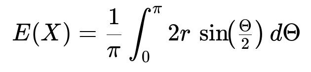
E(X) = (1/π) ∫[0..π] 2r sin(Θ/2) dΘ = (4r/π) ∫[0..π/2] sin(x) dx = (4r/π).

That integral yields 4r/π, which is approximately 1.273r.

Next, E(X²) = (1/π) ∫[0..π] (2r)² sin²(Θ/2) dΘ = (8r²/π) ∫[0..π/2] sin²(x) dx = 2r².

Hence Var(X) = E(X²) − [E(X)]² = 2r² − (4r/π)². This gives the standard deviation:

σ(X) = sqrt(2r² − 16r² / π²) = r sqrt(2 − 16/π²) ≈ 0.616r.

Comprehensive Explanation

Geometric Interpretation

We have a circle of radius r with center O. Let Q be a fixed point on the circle, and let P be a randomly chosen point on the circumference. Draw radii OQ and OP. The angle between OQ and OP (call it Θ) measures how far P is around the circle from Q. Because P is chosen uniformly on the circumference, Θ is uniformly distributed between 0 and π (not 2π, because reflecting P across Q simply yields the same chord length).

From basic geometry of circles, the chord length X between points P and Q is related to Θ by:

Here, X is the chord connecting P and Q, and Θ is the central angle subtended by that chord.

Expected Value of X

Because Θ is uniform on [0, π], we have:

It is often convenient to use x = Θ/2 as a substitution. Then as Θ goes from 0 to π, x goes from 0 to π/2, and dΘ = 2 dx. So:

E(X) = (2r/π) ∫[0..π] sin(Θ/2) dΘ becomes E(X) = (2r/π) · 2 ∫[0..π/2] sin(x) dx = (4r/π) ∫[0..π/2] sin(x) dx.

We know ∫[0..π/2] sin(x) dx = 1. Hence:

E(X) = (4r/π) × 1 = 4r/π.

In decimal form, 4/π is approximately 1.273, so E(X) ≈ 1.273r.

Expected Value of X²

Similarly, for the second moment E(X²), we do:

That becomes:

E(X²) = (1/π) ∫[0..π] 4r² sin²(Θ/2) dΘ = (4r²/π) ∫[0..π] sin²(Θ/2) dΘ.

With the same substitution x = Θ/2, the bounds on x go from 0 to π/2, and dΘ = 2 dx. Thus the integral becomes:

E(X²) = (4r²/π) · 2 ∫[0..π/2] sin²(x) dx = (8r²/π) ∫[0..π/2] sin²(x) dx.

Next, recall the integral of sin²(x) from 0 to π/2 is π/4. Substituting that in:

E(X²) = (8r²/π) × (π/4) = 2r².

Variance and Standard Deviation

The variance of X is Var(X) = E(X²) − [E(X)]² = 2r² − (4r/π)². Simplify:

(4r/π)² = 16r² / π²,

so:

Var(X) = 2r² − 16r² / π².

Hence the standard deviation is:

Numerically, sqrt(2 − 16/π²) ≈ 0.616, so σ(X) ≈ 0.616r.

Potential Follow-up Questions

1) Why is Θ uniform on [0, π] rather than [0, 2π]?

When we choose a random point P on the circle, it is indeed uniformly distributed over the full 2π range in angle. However, the chord length X depends on the absolute difference in angle between P and Q, which effectively ranges from 0 to π because the chord length is the same if P is clockwise or counterclockwise from Q. Indeed, if you let the angle range up to 2π, half of those angles would represent the same chord length. Thus restricting Θ to [0, π] properly captures every chord length possibility exactly once.

2) What happens if r = 0 or if r is extremely small or extremely large?

If r = 0, the circle collapses to a point. Then X = 0 deterministically, with expectation 0 and standard deviation 0. For very large r, the formulas still hold. E(X) just scales with r, and the standard deviation also scales with r. This linear scaling by r is natural for chord lengths, because chord geometry depends only on ratios to the circle’s radius.

3) Can we simulate this in Python quickly to check the result?

Yes. We can directly generate many random angles (in the [0, 2π] range, for instance), compute chord lengths relative to a fixed Q at angle 0, and then take means and standard deviations. A brief example:

import numpy as np

def simulate_chord_stats(r, n_samples=10_000_000):
    # Q fixed at angle 0 for convenience
    angles = 2 * np.pi * np.random.rand(n_samples)
    # Chord length: X = 2r * sin(|angles|/2), but we can mod to [0, pi]
    # angle_diff effectively in [0, pi]
    angle_diff = np.abs(angles - 0)
    angle_diff = np.where(angle_diff > np.pi, 2*np.pi - angle_diff, angle_diff)
    # Now compute chord length
    X = 2*r * np.sin(angle_diff/2)
    return X.mean(), X.std()

r_test = 1.0
mean_est, std_est = simulate_chord_stats(r_test)
print("Empirical mean:", mean_est)
print("Empirical std:", std_est)

This simulation will produce numerical estimates close to E(X) = 4r/π and σ(X) ≈ 0.616r if n_samples is large enough.

4) How could we approach this problem if the distribution of P was not uniform on the circumference?

If P were chosen in some other manner (e.g., uniformly in the area of the circle, or with some non-uniform distribution over the circumference), the angle Θ might not be uniform. We would need to derive the distribution for Θ or X accordingly, and then integrate to find the expectation and variance under that distribution. The uniform-on-the-circumference assumption is central to guaranteeing that Θ is uniform on [0, π].

5) Are there any connections to well-known probability problems involving circle chords?

Yes. There are several famous paradoxes, such as Bertrand’s paradox, which explores the different ways of defining a “random chord.” The question here specifically picks a chord determined by randomly choosing a point on the circumference. This leads to a well-defined distribution for chord lengths (related to Θ being uniform on [0, π]). But different definitions of “random chord” (e.g., picking two random points in the circle’s interior, picking midpoint in the circle, etc.) yield different distributions, demonstrating that “random chord” can be interpreted in multiple ways.

Below are additional follow-up questions

1) Could we derive E(X) and Var(X) without using direct integration?

One potential approach is to use geometric probability arguments or known results about chord lengths. For instance, it is known (via geometric probability) that when a chord is determined by choosing a point P uniformly on the circumference relative to a fixed point Q, the midpoint of that chord is distributed in a certain radial pattern inside the circle. By carefully analyzing how far that midpoint can be from the center, one can find the mean chord length without explicitly computing trigonometric integrals.

However, such geometric approaches often circle back to ideas very similar to the integral approach. In one variation, we note that the midpoint of a chord with fixed endpoints Q and P is at some distance from the circle center O, and the distribution of that distance can be used to deduce chord-length statistics. The advantage is that sometimes it sidesteps dealing with trigonometric integrals directly, but the level of conceptual difficulty is generally the same.

A subtle pitfall is that one must avoid mixing up different definitions of “random chord.” If we pick a chord by choosing any two random points on the circumference, that distribution differs from choosing one point randomly in relation to a fixed point. So, carefully specifying which random process is used is crucial. Otherwise, the “no-integration” approach could be incorrectly applied and yield inconsistent results.

2) How does this result generalize if we pick more than one random point P relative to Q?

If we consider multiple random points P1, P2, …, Pn on the same circle (each chosen independently), each chord QiPi (with Q fixed) will be distributed identically to the chord QP in the original problem. Hence each chord length Xi = |QiPi| has the same distribution as X. In such a scenario, the set of chord lengths {X1, X2, …, Xn} each follows the same distribution with mean 4r/π and standard deviation approximately 0.616r.

A more subtle question is whether these chord lengths are independent from each other. If the points Pi are chosen independently around the circumference, then each Xi is marginally distributed in the same way, but there are correlations (for instance, if you know P1 is close to Q, it does not necessarily provide direct information about where P2 is, but if constraints or sampling schemes are introduced that couple the points, the independence could be lost).

Pitfalls here include mixing up identical distribution with independence: the chord lengths are identically distributed but might not be strictly independent if the points are not chosen independently. Also, if we pick the n points by partitioning the circumference into equal arcs (deterministically or systematically), we lose the uniform randomness assumption.

3) Does this result hold if the radius r is itself random?

Sometimes, in real-world scenarios, we might not know r exactly but rather treat it as a random variable in a hierarchical model (e.g., the circle’s size might vary from one trial to another). In that case, the chord length X given r is still 2r sin(Θ/2), but now r is also uncertain. One could compute E(X) by conditioning on r:

E(X) = E [ E(X | r) ].

Since we know E(X | r) = 4r/π, it follows that E(X) = (4/π) E(r). The variance becomes more complicated because we also have the randomness of r. We would use:

Var(X) = E [ Var(X | r) ] + Var [ E(X | r) ].

Inside E[ Var(X | r) ], we have the expression for Var(X | r) = 2r² − 16r² / π². Meanwhile, E(X | r) = 4r/π. So we would need to incorporate the distribution of r into these formulas.

A major pitfall is forgetting to apply the law of total expectation and the law of total variance properly. If we simply plugged in E(r) for r in the chord length formulas, we would ignore the variance contributed by the random radius.

4) What if we only allow P to lie on a certain arc rather than the entire circumference?

If P is constrained to lie on an arc of length L < 2πr, then Θ will not be uniform on [0, π] in the same sense anymore. The effective distribution of the subtended angle changes because the chord can only come from a portion of the circumference. Consequently, the expected chord length E(X) could differ significantly.

The main approach to handle that scenario is to parameterize the arc in terms of the central angle it spans (say it goes from 0 to α, where α < 2π) and determine the induced distribution on the chord length. The ratio α / 2π would describe the fraction of the circumference used. Then we compute integrals or rely on geometric transformations for chord lengths within that arc.

An important subtlety: if the arc is small, the chord length distribution skews toward smaller values, because P will be close to Q. Another subtlety is that as α approaches π, we start to approximate the original distribution fairly well, but we must carefully set up the integral that respects the arc’s location relative to Q.

5) How would measurement noise affect the observed chord length distribution?

In practical scenarios (e.g., in computer vision, or in real-world geometry measurement devices), you never measure X perfectly. Suppose we measure X with additive Gaussian noise Z with mean 0 and standard deviation δ (for instance, from sensor error). Then the observed chord length would be X_obs = X + Z.

Its distribution is then the convolution of the chord length’s distribution with the noise distribution. While the mean of X_obs would still be 4r/π if the noise has zero mean, the variance of X_obs would be Var(X) + δ². If the noise is large enough (δ ≫ r), the chord’s intrinsic geometry might be overshadowed by the measurement noise, making it harder to detect the original chord-length distribution.

A pitfall here is failing to separate intrinsic geometric variability from measurement variability, leading to erroneous conclusions about the circle radius or the underlying geometry if we assume no noise in our model.

6) How does the distribution of X relate to the distribution of the angle Θ/2?

Since X = 2r sin(Θ/2), we can view the random variable X as a monotonic transformation of Θ/2 on [0, π/2]. If we wanted the probability density function f_X(x), we could derive it from the uniform distribution of Θ on [0, π]. Because Θ/2 ranges over [0, π/2], the PDF for x can be found by the standard transformation of random variables:

dX/d(Θ/2) = 2r cos(Θ/2), so f_X(x) = f_{Θ/2}(u) / |dX/du| evaluated at u = arcsin(x/(2r)).

This yields a PDF that is 1 / (π √(1 − (x/(2r))²)) for x in [0, 2r], illustrating a semicircle-like shape in the distribution for the random chord length.

A subtlety is that one must carefully handle boundary conditions: the chord length can never exceed 2r, and so the PDF has support only on [0, 2r]. Another subtlety is the factor-of-2 difference in the bounds for Θ versus Θ/2. Mistakes often arise if we do not keep track of that difference.

7) How would the result change if we fixed two different points Q1 and Q2, and chose P from the circumference uniformly at random?

Now the problem has two fixed references on the circumference, and we measure chord lengths P to Q1 and P to Q2. Each chord length alone would still follow the same distribution as the original chord QP (assuming we measure them separately). However, if we start asking joint questions—for instance, “What is the correlation between X1 = |PQ1| and X2 = |PQ2|?”—the random variables will not be independent because a given P that is near Q1 might also be near or far from Q2 depending on the geometry.

The distribution of each chord length individually remains the same (with mean 4r/π, standard deviation ~0.616r), but together they have a non-trivial joint distribution. A common pitfall is to assume that if each chord length has the same distribution, they must be uncorrelated. That is not necessarily true: the geometry can induce significant correlation.

8) Can we extend these ideas to higher-dimensional analogs, such as random distances between points on an n-sphere?

Yes. The chord interpretation generalizes to “random geodesics” on spheres or higher-dimensional manifolds. For instance, on the surface of a 2-sphere (Earth-like surface), the “chord” might be replaced by the great-circle distance between two random points. However, the distribution becomes more complex, and we often rely on known results for the distribution of chord lengths in higher dimensions or geodesic distances.

A direct extension of the geometry would be: pick one point Q on the surface of an n-sphere of radius r, then pick another point P uniformly on that n-sphere. The distribution of the Euclidean chord length X = ‖P − Q‖ in R^{n+1} can be computed from the spherical geometry. You would use that the angle between Q and P is uniform, but in higher dimensions the relationship between uniform distributions on the sphere and the angle is more subtle.

Pitfalls revolve around mixing up geodesic distance on the sphere with Euclidean distance in the ambient space. Also, there are complexities in the measure of uniform distribution on higher-dimensional spheres that differ from the 2D circle case. Failure to handle these geometric nuances can yield incorrect generalizations.