
ML Interview Q Series: Calculating Win Probability in a Two-Lead Game Series using Gambler's Ruin.

Browse all the Probability Interview Questions here.
35. Alice and Bob are playing a game until one has 2 more round-wins than the other. With probability p, Alice wins each round. What is the probability Bob wins the overall series?
Detailed Explanation of the Reasoning
We want to find the probability that Bob eventually gets 2 more cumulative wins than Alice before Alice gets 2 more wins than Bob. Let p be the probability that Alice wins each round, and thus 1−p is the probability that Bob wins each round. Because rounds are played repeatedly until one player leads the other by exactly 2 more wins, we can model the difference in total wins as a (one-dimensional) Markov chain or random walk.
Define the difference in wins after each round as:
difference = (Bob's total wins) − (Alice's total wins)
Initially, difference = 0. After each round:
• difference → difference + 1 with probability 1−p (Bob wins) • difference → difference − 1 with probability p (Alice wins)
We are interested in the probability that this difference eventually reaches +2 (Bob is 2 ahead) before it reaches −2 (Alice is 2 ahead). This is a classic gambler's ruin problem with absorbing states at +2 and −2.
When p ≠ 0.5, the known gambler’s ruin formula for a random walk that starts at 0 and moves +1 with probability 1−p and −1 with probability p can be adapted to the boundaries +2 and −2. The result of that analysis yields a probability that Bob’s lead hits +2 before −2 given by:

When p = 0.5, one can also use the symmetry of a fair random walk to show that the probability Bob reaches +2 before −2 (starting at 0) is 0.5, which is consistent with substituting p = 0.5 into the closed-form expression above:

Hence, the final probability that Bob wins the overall series (meaning he is the first to get 2 more total wins than Alice) is:

This formula can be further verified by checking corner cases:
• If p = 0, meaning Alice never wins a round, Bob trivially wins with probability 1. • If p = 1, meaning Alice always wins every round, Bob’s probability of ultimately winning is 0. • If p = 0.5, as mentioned above, the probability is 0.5.
These edge cases match the direct intuition for the problem.
Implementation Example (Simulation in Python)
One could perform a Monte Carlo simulation to empirically verify the above result. The random walk logic can be implemented as follows:
import random
import numpy as np

def simulate_bob_wins(num_simulations=10_000_000, p=0.3):
    # p is probability Alice wins a round
    # q is probability Bob wins a round
    q = 1 - p
    bob_wins_count = 0

    for _ in range(num_simulations):
        difference = 0
        while abs(difference) < 2:
            # random() < p => Alice wins
            if random.random() < p:
                difference -= 1  # difference = Bob - Alice, so Alice's win => difference -= 1
            else:
                difference += 1  # Bob's win => difference += 1

        if difference == 2:
            bob_wins_count += 1

    return bob_wins_count / num_simulations

# Example usage:
p = 0.3
estimated_probability = simulate_bob_wins(num_simulations=100_000, p=p)
theoretical_probability = ((1-p)**2) / ((1-p)**2 + p**2)

print("Estimated Probability Bob Wins:", estimated_probability)
print("Theoretical Probability Bob Wins:", theoretical_probability)
By running a sufficiently large number of simulations, the estimated probability will approach the theoretical value.
Why the Gambler’s Ruin Formula Applies
The essential insight is that at every step of the game, Bob either goes up by one win (with probability 1−p) or down by one win (with probability p). If we label Bob’s lead as a “fortune,” then Bob’s “fortune” is +2 if he wins the series and −2 if he loses. The random walk stops as soon as Bob’s fortune reaches +2 or −2. Because each round is independent and the probability does not change over time, the gambler’s ruin analysis for a one-dimensional random walk directly applies.
Further Discussion of the Underlying Math Expression

What if the probability of winning each round changes over time?
In many real-world scenarios, the probability of winning a “round” might be dynamic. For instance, Alice might improve over time, or the game’s environment might favor Bob at certain points. If the probability p is not constant, the standard gambler’s ruin style formula no longer directly applies. One must then consider a more general Markov chain where transition probabilities can change with each step. In that case, one could:
Use dynamic programming: Instead of a static closed-form expression, define the probability of eventually reaching +2 or −2 starting from a given difference, accounting for the stage-dependent probabilities.
Apply simulation: One might resort to a simulation-based approach for more complicated or time-varying probabilities. By repeatedly simulating the process with the changing probabilities, one can obtain an empirical estimate.
Pitfall: The closed-form solution derived above relies on time-homogeneous transition probabilities. Changing them invalidates the simple gambler’s ruin approach.
How can we interpret or derive this formula from first principles without the gambler’s ruin knowledge?
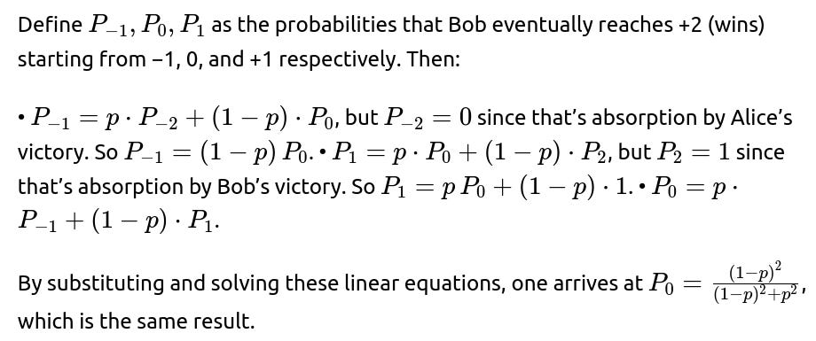
One way is to reason about states and their transition probabilities. Enumerate states −1, 0, +1 for the difference, ignoring the absorbing states −2 and +2 except as exit points. Solve the system of linear equations that arise from the condition that the probability of eventually reaching +2 from each non-absorbing state must reflect the transition probabilities:
What is the significance of the fair-random-walk case p = 0.5?
In a fair game (p = 0.5), the probability that Bob eventually obtains a lead of 2 before Alice obtains a lead of 2 is 0.5. This is because with a truly fair random walk, there is a symmetric chance for either side to eventually pull ahead by 2. It highlights a well-known gambler’s ruin principle: if the probabilities of stepping left or right are equal, from the starting point 0 and symmetrical absorbing states at +a and −b, the chance to hit +a before −b is the ratio of the initial distance from −b to the total distance between −b and +a. Here, that fraction is 2 / (2+2) = 1/2.
A common pitfall: Some may mistakenly think that if p = 0.5, each side has an equal chance of being ahead at each step, or that the chance might be 1 because eventually, someone must get ahead by 2. The correct reasoning is to observe that the event is symmetrical and each side has the same probability.
Could one compute the expected time to completion?
Yes, one can compute the expected number of rounds until either player is 2 ahead. In the gambler’s ruin setting, one can find the expected hitting time for a 1D random walk to be absorbed at +2 or −2 starting from 0. The expected time can be derived but involves more complicated sums than the basic probability of absorption. Generally, the expected time might be infinite for a fair random walk if the boundaries are very far away, but with boundaries only 2 steps away in each direction, it remains finite. The exact expression can be found through standard random walk hitting time calculations, though interviewers typically focus on the probability of eventually winning rather than the expected duration.
How does this result connect to real-world problem statements in Machine Learning or other fields?
Markov processes or random walks with absorbing states frequently appear in:
• Markov Decision Processes (MDPs) for reinforcement learning (though typically one has control over actions, probabilities can be similarly analyzed). • Genetic algorithms or evolutionary strategies when modeling fixation probabilities (the probability that a certain gene variant fixes in the population). • AB testing with sequential updates, though typically AB testing has more elaborations (like stopping rules). • Stock market or other gambler’s ruin analogies in finance.
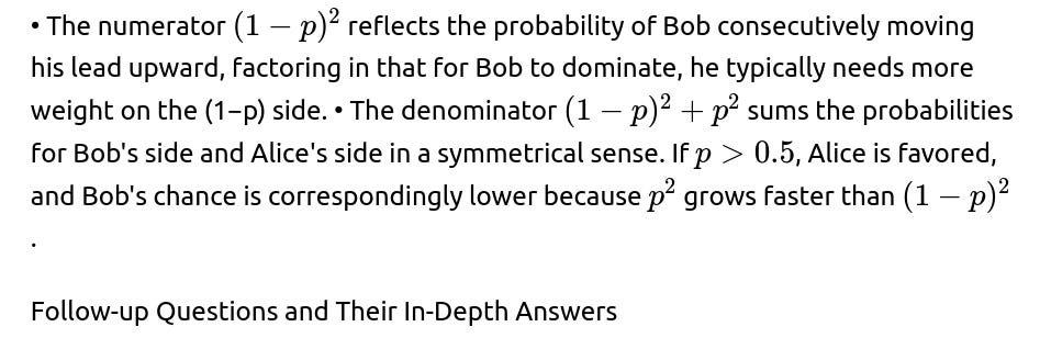
When p represents a performance advantage (say, the probability that model A outperforms model B in a sequence of tests), the formula gives the chance that B “wins the competition” by beating A in enough consecutive trials to lead by 2. Understanding such random walk or gambler’s ruin arguments helps ML practitioners reason about iterative processes, repeated tests, or repeated “battles” in a multi-agent system.
If we needed to generalize to the case where the game stops when a difference of k is reached, how does the formula change?
For a random walk that increments with probability q = (1−p) and decrements with probability p, from a starting difference of 0, the probability of eventually hitting +k before −k is given by:


But one must track the offset that 0 is actually k away from the negative boundary. Solving a system of linear equations for a general boundary ±k is typically the easiest route to avoid confusion. The core takeaway is that for +k vs −k, a standard gambler’s ruin formula applies, with p replaced by the probability of stepping “down” and q replaced by the probability of stepping “up.”
Are there any hidden assumptions?
One assumption is that each round is independent and identically distributed with probability p for Alice. Another assumption is that the process continues indefinitely until one player is ahead by 2. We also assume p is constant over all rounds. If these assumptions break, the formula changes.
Another subtlety is the possibility that the game could never end if probabilities were such that one might keep oscillating. However, for 0 < p < 1, and the random walk being a 1D unbiased or biased step, we can show that eventually it almost surely hits one of the boundaries ±2. For 0 < p < 1, a random walk in one dimension with absorbing boundaries at ±2 has a probability of 1 of eventually being absorbed, so the sum of probabilities (Bob’s or Alice’s final victory) must be 1.
Does the formula still hold if the rounds are not memoryless?
If the probabilities of Bob or Alice winning each round depend on the entire history or on how many wins they already have, one must revert to a more general state-based approach. Memorylessness is key in using the gambler’s ruin style approach. If memorylessness is violated, one might:
• Formulate the entire game as a Markov chain with an enlarged state that tracks the history needed to determine p at each step. • Use dynamic programming or direct simulation to estimate the final probability.
As soon as you change the probability of winning from p to some function of the current difference or the past, you must handle it with more advanced methods.
What if we wanted to confirm these probabilities quickly in an interview without code?
A quick mental or paper-based Markov chain argument can be done by labeling states for difference = −1, 0, +1 and applying the boundary conditions at −2 and +2. Set up linear equations for the probabilities of eventually hitting +2 from each state, and solve them. This is a compact approach that often impresses interviewers since it demonstrates a fundamental understanding of how to handle absorbing Markov chains.
Below are additional follow-up questions
What if we only track a partial count of wins for each player, rather than all past rounds?
One scenario is where we only keep track of recent rounds or the most recent lead changes, perhaps due to storage constraints or because old rounds become “irrelevant.” In that case, the Markov property of the difference in total wins is broken, and we no longer have a memoryless process in the standard gambler’s ruin sense. Instead, we have a situation closer to a partially observed Markov process, or even a semi-Markov process, depending on how the partial information is retained.
To analyze it:
• You could maintain a truncated state space, which tracks only the last few leads or partial totals. This might be artificially restricting the system’s memory to some finite range of values. • The probability of eventually obtaining a +2 lead or −2 lead might need a custom dynamic programming approach or even simulation. Each partial state transitions to another partial state based on newly observed round outcomes. • A key pitfall is that the partial record might lose crucial information about how many total leads have accumulated so far, which can affect the probability of eventually hitting +2 or −2. • In practice, you might do a state expansion to keep enough memory for the Markov property to hold (for example, store the current lead plus some relevant context) or revert to a Monte Carlo simulation, which can handle complex logic about how partial states evolve.
Edge Cases:
• If the partial tracking is too small, you can inadvertently change the fundamental probability of absorbing states because you might “forget” that Bob or Alice was previously closer to +2 or −2. • You might wrongly conclude the game continues when in fact one player is effectively guaranteed to reach +2 or −2 based on older but crucial data.
How does a small but non-zero probability of a tie in each round affect the analysis?
Consider that each round can end in three possible outcomes: Alice wins, Bob wins, or a tie with a small probability t. Then the probability of Alice winning becomes p, Bob winning becomes q = 1−p−t, and tie becomes t. The game presumably only progresses (in terms of changing the difference) on a non-tie result. If we still say the game stops when one player has exactly 2 more wins than the other, we have to incorporate these ties into our model.
Key points:
• Ties do not change the difference in wins but do consume a round. Thus, the random walk “pauses” whenever a tie occurs. • Because ties don’t move us closer or further from ±2, they increase the expected length of the game. The probability of eventually ending the game might remain 1 (assuming p + q > 0, so eventually wins happen), but the presence of ties prolongs the time to absorption. • The gambler’s ruin style formula can be adapted if we condition on a non-tie outcome. Specifically, if a tie occurs with probability t, then upon a non-tie result, the probability of an Alice win is p/(p+q) and Bob win is q/(p+q), where p+q < 1. The random walk transitions only when a non-tie is observed. • The probability of Bob eventually getting +2 can be computed using the “rescaled” probabilities p/(1−t) and q/(1−t), treating ties as neutral events that simply delay the process. The standard gambler’s ruin formula becomes:

This is because effectively, the ratio q : p is what drives the random walk transitions.
Potential Pitfalls:
• Failing to rescale p and q by 1−t can lead to incorrect probabilities for hitting ±2. • If t is extremely large (close to 1), the game can take a very long time to conclude. Real systems might impose a cutoff after a certain number of ties, leading to a new boundary condition (e.g., “end in a draw if we exceed N total rounds”). In that scenario, you must incorporate that additional absorbing state for a “draw.”
Could numerical instability occur for extreme values of p?
Yes, numerical instability can crop up when p is very close to 1 or 0:
• If p is extremely close to 1, then Bob’s probability of eventually winning should be very close to 0. But evaluating the expression

might lead to floating-point underflow or precision issues if p is near 1. For instance, if p=0.99999999, then p^2 is about 0.99999998, and (1−p) is around 1e−8, so (1−p)^2=1e−16, which can easily cause floating-point underflow in standard double-precision if not handled carefully. • Similar issues arise if p is near 0. In that case, (1−p) might be close to 1, so the numerator becomes close to 1, and the denominator is also close to 1, but any small floating-point error might cause a difference in the final computed fraction.
Pitfall Mitigation:
• One approach is to implement the formula with a check for boundary conditions, such that if p < some epsilon, we simply return 1 for Bob’s probability. Similarly, if p > 1−epsilon, we return 0. • Alternatively, rewrite the formula in a numerically stable way, such as factoring out the larger of (1−p)^2 or p^2 to reduce floating-point overflow or underflow.
What if the game is subject to an external time limit or a maximum number of rounds?
If the game must end by a certain round limit N, with no winner declared if neither player is ahead by 2 by that time, the problem changes:
• Now the states ±2 remain absorbing, but there’s also a new terminal time limit. If the random walk (difference in wins) is in the set {−1, 0, +1} after N rounds, we reach a new “draw” absorbing state. • The probability that Bob eventually wins before round N is strictly less than the infinite-horizon gambler’s ruin probability, because there is a possibility that no player gets a +2 lead by round N. • Analyzing it requires either enumerating the distribution of possible differences after each round up to N or using a dynamic programming approach that tracks the probability of being at each difference −1, 0, +1 after k rounds. By summing the probability mass that eventually reaches +2 before hitting N rounds, you get Bob’s probability of winning.
Edge Cases and Pitfalls:
• If N is too small, it might be impossible for either player to accumulate a +2 lead. Then the probability is 0 for both Bob and Alice, with the entire probability going to the “draw” state. • If p is extremely close to 0.5 and N is moderate, a large fraction of repeated sequences can end up with no +2 lead by the time N is reached.
Does the formula or approach change if the "difference" must be exactly 2 consecutive wins?
Sometimes, a question might be misinterpreted as “Bob needs to win 2 rounds in a row,” rather than “Bob needs 2 total more wins.” If the requirement is specifically two consecutive wins, that is a different problem:
• The states revolve around whether Bob’s last round was a win, whether Bob has 1 consecutive win, and so on. • The standard gambler’s ruin formula does not apply because we are not tracking a difference in totals but the length of the current consecutive-win streak. • In that consecutive-win scenario, you would have states S0 (no consecutive wins), S1 (1 consecutive win for Bob), and absorbing state S2 (2 consecutive wins for Bob). There would also be an absorbing state for Alice if the condition changes to “Alice must achieve 2 consecutive wins” or “Alice must get 2 more total wins,” etc.
Pitfalls:
• Failing to differentiate between “2 more total wins” and “2 consecutive wins” can lead to the incorrect application of gambler’s ruin logic. • The probability for Bob to get 2 consecutive wins might be simpler or more complicated depending on whether Alice has her own target. If both want 2 consecutive, we track Bob’s consecutive count and Alice’s consecutive count, resetting if the other side wins a round.
Can we transform this problem into a standard gambler’s ruin with different states?
Yes, one subtlety is that the boundaries are ±2, but we can reindex the states to be 0, 1, 2, 3 where the difference = −1 corresponds to state 1, difference = 0 corresponds to state 2, difference = +1 corresponds to state 3, difference = −2 is an absorbing state 0, difference = +2 is absorbing state 4, etc. The probability transitions remain p or 1−p for stepping to adjacent states, but the boundaries become 0 and 4.
Why do this?
• Sometimes it’s more intuitive or consistent with standard gambler’s ruin references that define 0 and M as boundaries with the random walk starting somewhere in between. • The reindexing doesn’t change the answer but might simplify the linear algebra approach for solving for the absorbing probabilities.
Pitfalls:
• Off-by-one errors if you incorrectly label the states or mismatch them with the difference in wins. • Overcomplicating the problem if the direct difference-based approach is simpler for your mental model.
What about the probability that Bob leads by 2 at any point (not necessarily for the first time)?
A tricky variation is to ask: “What is the probability that Bob’s lead is at least +2 at any point in time, not necessarily the first time the difference hits +2?” That’s slightly different because:
• The original problem states the game ends as soon as the difference is +2 or −2. That forces us to focus on the first hitting time to ±2. • If we are interested in whether Bob’s lead ever reaches +2 (even if the game doesn’t end there or if we allow the game to continue for more than that moment), we’re dealing with an event that can happen at any round, possibly multiple times, if the game continued hypothetically. • For a standard gambler’s ruin approach that stops the process immediately at ±2, the probability of Bob eventually hitting +2 is exactly the probability that Bob “wins” the game. But if the game didn’t stop, we might have a scenario where Bob’s lead hits +2 but then Alice eventually surpasses him. That scenario is typically disallowed in the original question because the game ends as soon as ±2 is reached.
Edge Cases:
• If the game did not have absorbing boundaries, the question about the random walk “ever” hitting +2 can be answered by separate results from random-walk theory (the probability that a simple symmetric or biased random walk eventually hits a certain boundary if the walk is infinite). For a biased walk that drifts downward, it might never reach +2. • For an unbiased random walk (p=0.5), the probability of eventually hitting any finite boundary in an infinite walk is 1, though the expected time might be infinite.
How to handle the scenario where p is unknown and must be estimated on the fly?
In many real-world settings, we might not know p ahead of time. We could observe outcomes of initial rounds and update our estimate of p with a Bayesian or frequentist approach. Then we have a few possible ways to proceed:

What if there's a payout that depends on intermediate leads, not just who eventually wins by 2?
Sometimes, the game might award partial payouts for partial leads along the way. For instance, if Bob is leading by 1 at certain checkpoints, Bob might get a small reward. In that scenario:
• The final objective is not solely to reach +2 but also to maximize expected payout over the entire trajectory. • We move beyond the basic gambler’s ruin framing and instead consider the expected sum of payouts across states visited. This is reminiscent of Markov Reward Processes in reinforcement learning. • The probability that Bob eventually hits +2 is still relevant, but you also have to incorporate partial payoffs for being in the +1 state at different times.
Pitfalls:
• Under this new payoff structure, it’s possible that Bob might prefer strategies (if he has any control, which in a purely random setting he doesn’t) that increase the likelihood of being in a +1 state more frequently even if that reduces the final chance of reaching +2. • If the game is purely random with probability p, then Bob can’t strategically alter outcomes, so we only analyze expected payoffs by summing up the fraction of time spent in each positive lead state.
How does one handle correlated round outcomes?
If the outcome of one round depends on who won the previous round (e.g., a psychological momentum effect), then p can no longer be treated as constant from round to round. Possible ways to model it:
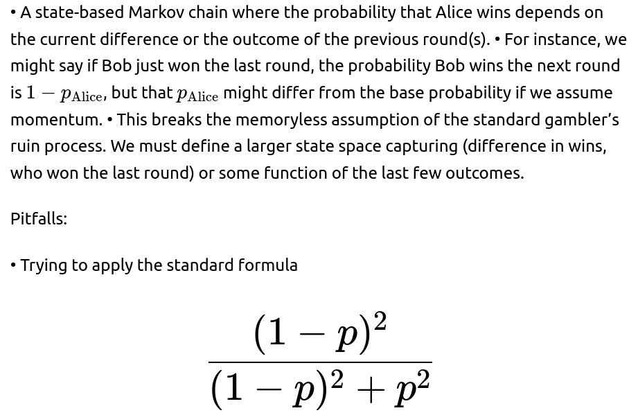
when momentum or correlation is present is incorrect. That formula specifically assumes i.i.d. Bernoulli trials with success probability p for Alice each time. • For correlated rounds, one either sets up a custom Markov chain with more states or uses simulation to approximate the probability that Bob eventually gets to a lead of +2.
Could we extend the approach to n players, where the series ends once any player is 2 wins ahead of all others?
In a scenario with more than two players—say Alice, Bob, and Carol—each round might have a single winner among the three, or some other structure. The condition might be that a player is 2 wins ahead of each of the other two:
• The state now becomes the vector of wins (or differences) for the players. For example, we could track (wins by Alice, wins by Bob, wins by Carol), or differences between pairs. • The absorbing condition is that any one player’s number of wins is at least 2 above each other player’s wins. That means (A − B) ≥ 2 and (A − C) ≥ 2 for Alice’s absorption, etc. • Standard gambler’s ruin results do not extend directly, and we might need a multi-dimensional random walk approach. The probability of each player eventually achieving a 2-win lead over everyone else can be found via multi-dimensional Markov chain analysis or simulation.
Pitfalls:
• The dimensionality grows quickly, making a direct enumerative approach expensive. For large differences or more players, it becomes computationally challenging. • If the probability distribution among players is not uniform (e.g., Alice has probability p, Bob has probability q, Carol has probability r with p+q+r=1), the transitions in each step are more complicated.