
ML Interview Q Series: Calculating Alpha Particle Emission Probabilities using Poisson Distribution

Browse all the Probability Interview Questions here.
Experiments by Rutherford and Geiger in 1910 showed that the number of alpha particles emitted per unit time in a radioactive process is a random variable having a Poisson distribution. Let X denote the count over one second and suppose it has mean 5. What is the probability of observing fewer than two particles during any given second? What is the P(X >= 10)? Let Y denote the count over a separate period of 1.5 seconds. What is P(Y >= 10)? What is P(X + Y >= 10)?
Short Compact solution
P(X ≤ 1) = e^(-5) (1 + 5) = 0.0404
P(X ≥ 10) = 0.0398
Since Y ~ Poisson(7.5), P(Y ≥ 10) = 1 - P(Y ≤ 9) = 1 - Σ(i=0 to 9) P(Y = i) = 0.5113
X + Y ~ Poisson(12.5), and P(X + Y ≥ 10) = 0.7986
Comprehensive Explanation
Poisson Distribution and Basic Properties
When we say X is Poisson(λ), it means that X is a discrete random variable counting the number of events (in this scenario, alpha particles emitted) in a fixed interval of time or space, with events occurring independently at a constant average rate λ. The probability mass function (pmf) of X is given by:
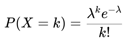
where:
λ is the average number of events in the given interval (mean rate),
k is the count of events (nonnegative integer),
e is the base of the natural logarithm.
In this problem:
We consider X as the Poisson-distributed count of alpha particles in 1 second, with λ = 5.
Probability of Observing Fewer Than Two Particles
“Fewer than two particles” means X ≤ 1. We calculate:
P(X ≤ 1) = P(X = 0) + P(X = 1).
Using the pmf:
P(X = 0) = (5^0 e^(-5)) / 0! = e^(-5).
P(X = 1) = (5^1 e^(-5)) / 1! = 5 e^(-5).
So P(X ≤ 1) = e^(-5) + 5 e^(-5) = e^(-5)(1 + 5).
Probability That X ≥ 10
For X ≥ 10, you can either compute 1 − P(X ≤ 9) or use tables/software to find the direct tail probability. The short solution gives this value as approximately 0.0398.
Y Over 1.5 Seconds
If Y is the count over a separate 1.5-second interval and the average rate is 5 particles per second, then for 1.5 seconds the mean is λ = 7.5. Thus Y ~ Poisson(7.5).
Hence: P(Y ≥ 10) = 1 − P(Y ≤ 9) = 1 − Σ(i=0 to 9) P(Y = i).
The short solution gives the final value as about 0.5113.
Sum of Independent Poisson Random Variables
A crucial property of independent Poisson random variables is that their sum is also Poisson, with the mean being the sum of their individual means. Since X ~ Poisson(5) and Y ~ Poisson(7.5), and X, Y are independent, X + Y ~ Poisson(5 + 7.5) = Poisson(12.5).
Therefore: P(X + Y ≥ 10) = 1 − P(X + Y ≤ 9).
The short solution indicates this probability is around 0.7986.
Practical Computation in Python
Below is a Python snippet illustrating how you could compute these probabilities with functions from the math module or from scipy.stats:
import math
from math import exp, factorial
from itertools import product
from scipy.stats import poisson

# Direct calculation for P(X <= 1) when lambda=5
p_x_le_1 = math.exp(-5)*(1 + 5)

# Using SciPy for P(X >= 10) for X ~ Poisson(5)
p_x_ge_10 = 1 - poisson.cdf(9, 5)

# For Y ~ Poisson(7.5)
p_y_ge_10 = 1 - poisson.cdf(9, 7.5)

# For X+Y ~ Poisson(12.5)
p_x_plus_y_ge_10 = 1 - poisson.cdf(9, 12.5)

print("P(X ≤ 1) =", p_x_le_1)
print("P(X ≥ 10) =", p_x_ge_10)
print("P(Y ≥ 10) =", p_y_ge_10)
print("P(X+Y ≥ 10) =", p_x_plus_y_ge_10)
This code uses the Poisson cumulative distribution function (CDF) poisson.cdf for an exact calculation.
What If The Interviewer Asks Further?
Why Does the Sum of Two Independent Poisson(λ1) and Poisson(λ2) Random Variables Become Poisson(λ1 + λ2)?
This is a well-known property of the Poisson process. Intuitively, each source of arrivals is independent, and if the average rate is additive, the overall combined arrival count is Poisson with the sum of the rates. Formally, it can be shown by convolving two Poisson pmfs or by the underlying property of the Poisson process that independent increments over disjoint time intervals have Poisson distributions with means that add up.
How Can We Approximate These Probabilities If λ Is Large?
When λ is large, the Poisson distribution can be approximated by a normal distribution with mean λ and variance λ. For X ~ Poisson(λ), a normal approximation would be Normal(λ, λ). In practice, for values of λ around 5 or 7.5, you might still get a fair approximation, but if λ were much larger (e.g., 50 or 100), the normal approximation often becomes more accurate. However, in modern practice, direct computation with software is typically straightforward even for moderately large λ.
Could the Time Intervals Overlap?
If two intervals overlap, the counts during that overlap are not strictly independent, so we cannot simply add Poisson rates for the overlap unless we carefully handle the shared portion. For example, if we have X for the first second and Y for the first 1.5 seconds (including that first second), then there is a 1-second overlap. In that case, X and Y are dependent, and we cannot immediately claim X + Y is Poisson(12.5). The standard property that the sum is Poisson(λ1 + λ2) only holds under independence (which typically means disjoint intervals for a standard Poisson process).
How to Estimate λ When It Is Not Given?
In practical settings, λ is often unknown and must be estimated from data. If you observe counts x_1, x_2, …, x_n from n independent, identical time intervals, the maximum likelihood estimate for λ is the sample mean (sum of observed counts / n). This is a fundamental property of the Poisson distribution: the sample mean is an unbiased and consistent estimator for the true rate.
How Could This Knowledge Be Applied to Real-World Scenarios?
Poisson distributions model many counting processes, such as the number of network requests arriving at a server, defect rates in manufacturing, or even goals scored in sports matches (under certain assumptions). Understanding the distribution helps in capacity planning, detecting anomalies (e.g., excessive counts in a given interval), or assessing the likelihood of rare high-count events.
Knowing how to calculate these probabilities directly, how to handle sums of counts over disjoint intervals, and how to approximate or simulate these events can be crucial for real-time systems monitoring, anomaly detection, or reliability calculations.
Handling Edge Cases and Practical Concerns
When λ is non-integer or intervals vary, you simply scale λ by the length of each interval (e.g., 7.5 for a 1.5-second interval if the rate is 5 events/second). If the intervals are not disjoint or independence is questionable, the sum may not be a pure Poisson distribution. In practice, always confirm that the Poisson assumptions (independence, constant average rate, no limit on possible events in an interval) are appropriate to the real-world process before applying the model.