
ML Interview Q Series: Calculating Expected Escape Time Through Probabilistic Looping Paths Using Expected Value Analysis.
Browse all the Probability Interview Questions here.
A miner must pick between two possible routes, where one option repeatedly loops him back to his starting point in 5 days, and the other takes him instantly to a fork in the road that has two further branches: one returns him to the start in 3 days, the other leads to safety in 1 day. If each path is equally likely, how many days on average will it take him to get out of the mine?
Comprehensive Explanation
The problem describes a random process where the miner is trying to escape a mine. He repeatedly makes choices among paths, with each choice having an equal probability (1/2) of being taken. We denote:
Path A: Takes 5 days, and then returns him back to the original starting point.
Path B: Takes 0 days to reach a junction. From this junction, there are two sub-paths:
Path B A: Takes 3 days, then returns him back to the original start.
Path B B: Takes 1 day to escape to safety.
He chooses between Path A and Path B with probability 1/2 each time he arrives at the start. If he goes down Path B, there is again a 1/2 chance to take the sub-path B A or sub-path B B. Once a path leads him back to the start, he has no memory of which path he took, so the process repeats indefinitely until he reaches safety.
To solve for the expected value E of the number of days spent before exiting, it is helpful to define two expected values:
E: The expected number of days starting from the initial point (the very start).
F: The expected number of days starting from the junction on Path B.
We can write down the core equations for E and F. First, from the start:
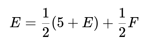
This reflects the fact that with probability 1/2 the miner chooses Path A (spends 5 days and returns to start, adding E again), and with probability 1/2 he chooses Path B (0 days to junction, then adds F).
Similarly, from the junction:
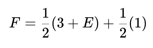
Half the time (1/2) he chooses Path B A, which takes 3 days and returns him to the start (adding E again), and half the time (1/2) he takes Path B B, which takes 1 day and leads to escape (no more days are added).
Below is a step-by-step outline of how to solve these equations:
From the second equation for F: F = (1/2)(3 + E) + (1/2)(1). Expanding: F = 1.5 + E/2 + 0.5 = 2 + E/2.
Substitute F into the first equation: E = (1/2)(5 + E) + (1/2)(2 + E/2). Multiply everything out: E = (5 + E)/2 + (2 + E/2)/2. E = (5 + E)/2 + (2/2) + (E/2)/2. E = (5 + E)/2 + 1 + E/4. Multiply both sides by 4 to clear denominators: 4E = 2(5 + E) + 4 + E. 4E = 10 + 2E + 4 + E = 14 + 3E. 4E - 3E = 14. E = 14.
Then, plugging E = 14 back into F = 2 + E/2 gives: F = 2 + 14/2 = 2 + 7 = 9.
Thus, the expected time before the miner reaches safety is 14 days.
Simulation Example in Python
A quick Monte Carlo simulation can help verify the above theoretical result. Below is an illustrative code snippet:
import random
import statistics

def simulate(num_runs=1_000_000):
    times = []
    for _ in range(num_runs):
        total_days = 0
        while True:
            # 50-50 chance for Path A or B
            if random.random() < 0.5:
                # Path A: 5 days, back to start
                total_days += 5
            else:
                # Path B: 0 days to junction, 50-50 for subpaths
                if random.random() < 0.5:
                    # Path B A: 3 days, then back to start
                    total_days += 3
                else:
                    # Path B B: 1 day, then exit
                    total_days += 1
                    break
        times.append(total_days)
    return statistics.mean(times)

average_days = simulate()
print("Estimated average days:", average_days)
Running this simulation many times will converge on an average close to 14 days, confirming the analytical solution.
What If the Probabilities Change?
If Path A or Path B were chosen with different probabilities (say p for Path A and 1-p for Path B), you could still define the equations for E and F accordingly, but they would now include these altered probabilities. The final expression for E would change, although the general solution approach would remain the same.
Follow-up Questions
How would you handle the situation if the paths took random amounts of time rather than constant times?
In that scenario, instead of each path taking a fixed number of days, each path would have a distribution of possible durations. The analysis would require taking the expectation of those random durations. Concretely, if Path A took X days on average and Path B had sub-paths that took Y and Z days on average, you would substitute those expected values into similar equations for E and F. However, you might also have to handle variances and use the law of total expectation carefully if the random times were to be combined with further random path choices.
Could the miner exploit any strategy to minimize time if he had partial memory?
If the miner had partial memory—for instance, if he could remember which path was taken on the previous choice—he could try to avoid repeating an unsuccessful path. This would change the Markov-like property of the process, because now the probability of choosing a given path is conditional on what happened before. With such memory, the expected time to exit could drop significantly, since he would not retry the same path and get stuck in loops repeatedly.
What if we allow the miner to place markings on the paths?
If the miner can mark paths he has traveled before, he could deliberately avoid repeating them. This again breaks the assumption that each path has the same probability of being chosen each time. With marking, after the first loop, the miner could always choose a path not previously taken. This would effectively eliminate the possibility of endless repeats, drastically reducing the expected time. In that setting, the problem becomes quite different, almost trivial, because once he tries Path A and sees it fails, he could systematically avoid it forever.
Why do we define a separate variable F for the junction?
Defining a separate expected value for the junction (F) allows us to handle sub-problems more systematically. When the miner arrives at the junction, the expected additional time from that point onward might differ from the expected time at the original starting point, because the available choices and their probabilities at the junction are different. This technique—breaking problems into sub-states and defining expected values for each sub-state—is a common approach in stochastic process analysis and dynamic programming.
Could you extend this logic to more complex networks of paths and junctions?
Yes. The same principle applies if the miner faces multiple junctions, each with different probabilities and path durations. You would define an expected time variable for each junction or state and set up a system of linear equations reflecting how the miner transitions among these states. Solving that system provides the overall expected time to reach an exit. In more complicated graphs, Markov chain methods or dynamic programming can be employed to handle the large number of states.
These types of extensions are common in real-world applications, such as analyzing average times in queueing networks or reliability problems in networks of systems. The key is consistently applying the law of total expectation to account for each possible transition.
Below are additional follow-up questions
How would the solution change if Path B’s two sub-paths do not have equal probabilities?
If the miner reaches the junction along Path B, there might be a different probability p for choosing Path B A and (1-p) for choosing Path B B. This changes the equation for F (the expected time from the junction). Specifically, instead of a 1/2 probability for each sub-path, the expected time at the junction becomes:
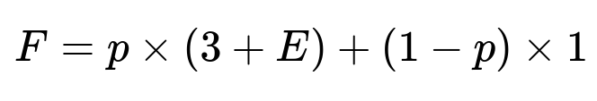
Because the miner returns to the start with probability p (spending 3 days first) and successfully escapes (spending 1 day) with probability (1-p). Once you have that new equation for F, you would plug it back into the expression for E. In other words, the general approach remains:
E = (1/2)(5 + E) + (1/2)F
but F changes to account for the altered probabilities. A key point is that the probability distribution for sub-paths within Path B is no longer symmetrical, so you must carefully handle p and (1-p).
A potential pitfall is neglecting to correctly adjust for these new probabilities when rewriting the expectation equations. Another subtlety might arise if p=0 or p=1, as this effectively reduces the problem to a single possible sub-path—an edge case that makes the loop or the immediate escape certain.
What if each subsequent journey down Path A or Path B takes slightly longer due to fatigue?
In this scenario, the time cost of traversing a path is not fixed but could increase with the number of attempts (for example, Path A might take 5 days on the first attempt, 5.5 on the second, and so on). The expectation calculation becomes more intricate because each return to the start no longer resets the travel time to a constant; the cost accumulates or changes dynamically.
One way to handle this is to introduce a new state variable representing how many times the path has been taken. Then, you would define E_n as the expected number of days to escape given that you have already taken n loops of Path A (or similarly Path B). This leads to a more complex system of equations with state-based transitions. For a purely linear fatigue effect, you could attempt to solve it analytically by summation of partial expected times. A common pitfall is accidentally treating each journey as if it still has a constant cost and ignoring how the times might be dynamically changing. Moreover, if the miner only experiences fatigue on certain paths, you have to keep track of which path caused the fatigue to ensure you are adjusting the correct time cost.
How could we accommodate a scenario where the miner obtains partial information about the path outcomes each time?
In a partial-information framework, maybe the miner notices certain landmarks that tell him he is going down Path A vs. Path B, or that he can detect an upcoming loop partway through. This partial observability fundamentally changes the model from a simple Markov chain to a Partially Observable Markov Decision Process (POMDP).
To tackle this, you would define beliefs or probabilities over which path you are currently on based on the observations. Then, the miner could choose different actions (like continuing forward or turning back) based on the updated belief state. A common subtlety is handling how the observation process interacts with the transitions—if the miner becomes more confident he is heading toward a loop, he might choose to reverse course, but that also has a cost in days. A key pitfall is failing to track how partial observations update beliefs about which path is which, leading to incorrect policies or expected time calculations.
What if there is a small chance that the miner never escapes (for instance, if Path B B occasionally fails to lead to safety and sends him back)?
If there is a nonzero probability of never escaping, the expected time could be infinite, depending on how these probabilities add up. For example, imagine that Path B B typically leads to safety but sometimes also loops back to the start. If those loopbacks happen with a small probability, you need to check whether the sum of probabilities for an infinite sequence of loops is large enough to make the expected time infinite.
A pitfall is overlooking the possibility that a seemingly small probability of repeatedly going in circles, over an unbounded number of attempts, can yield an infinite expectation. This scenario often arises in Markov chain analysis, where you must examine whether the chain has recurrent states (states you return to with probability 1 if you ever leave them). If a recurrent cycle cannot be escaped eventually, the expected escape time can become unbounded.
How does the analysis change if there is more than one possible exit and each path might lead to different exits?
Suppose there are multiple exits scattered around different paths. The miner’s process might then terminate when he reaches any exit. You would introduce separate states in your analysis for each exit and possibly distinct probabilities or times to travel among different junctions. The problem becomes a Markov chain with multiple absorbing states (the exits). Each path that leads to an exit is effectively an absorbing state with no further transitions. To find the overall expected time to absorption, you can set up the transition probability matrix for the chain and solve the fundamental matrix equation for absorbing Markov chains:
(N = (I - Q)^{-1} gives you the fundamental matrix, where Q is the transition matrix among the non-absorbing states).
One edge case arises if some of those exits are easier to reach but the miner might not choose them due to the random path selection mechanism. Another subtlety is if some exit states can only be reached from a subset of paths, so the chain structure may have multiple absorbing classes, and you have to compute the probabilities of ending in each class. This can get very complicated, and you have to be systematic to avoid mixing up the transitions.
What if the time to traverse a path is dependent on how recently the miner attempted that same path?
In certain realistic situations, if the miner returns to a path too soon, maybe a tunnel collapse or partial flooding has occurred, changing the travel time. This introduces memory into the process. The Markov property (which assumes the future depends only on the present state) no longer holds if the cost depends on past visits. One approach is to expand your state representation to include how long ago the miner took a particular path or how many times it has been taken in a row. This effectively increases the dimension of your state space and could make an analytical solution very challenging.
A key pitfall is trying to apply standard Markov chain techniques to a scenario that is no longer memoryless. You must incorporate that history into the definition of the state, or else you can incorrectly compute the expected time. Another subtlety is that if the cost can either increase or decrease unpredictably, you may need a full stochastic process model with time-series elements to track the changing conditions of each path.
How would outcomes differ if the miner could choose distinct paths with controlled probabilities each time rather than a strict 50-50 choice?
If the miner has partial control over which path to take, he might try a 70-30 split instead of 50-50, hoping to improve his average outcome. That transforms the problem into an optimization scenario, where the miner can pick a strategy of selecting Path A vs. Path B with certain probabilities each time he returns.
You would then define E as a function of the chosen probability q to take Path A (and 1-q for Path B) and minimize E with respect to q. You might find that the optimal policy is to pick Path B with probability 1 if it has a potential short route to safety—unless Path A also has some advantage.
A subtle pitfall is incorrectly assuming that always picking the path with the fastest possible route is optimal if there is some chance it might lead to a huge time penalty upon repeated cycles. You should properly weigh the expected time from each path instead of just picking based on the best short-term outcome. This can be an instance of the exploration-exploitation tradeoff, albeit in a simpler form.
What if Path B includes multiple junctions, each branching to different sub-paths, and the miner has to pick among them repeatedly?
In a more realistic labyrinth scenario, the miner might find multiple consecutive junctions each time he chooses Path B. This transforms the setup into a tree (or potentially a directed graph). You would assign a variable for the expected time from each node in the graph, including the start node, and write equations reflecting the possible transitions. The final solution emerges from solving this system of linear equations, where each node’s expected time depends on the times of the nodes it can transition to and the travel times along the edges.
An important pitfall is losing track of cycles if the miner can end up in a sub-junction that leads him back to a previous node (another loop). Handling those loops requires carefully ensuring that the equations reflect the probability of returning to the same node or moving to other nodes. A real subtlety arises when multiple loops exist, each with different travel times, and the probabilities of traveling among them might create complex cyclical patterns.
Does the approach differ if the travel times or path probabilities are time-varying (e.g., day vs. night changes in path accessibility)?
Yes, if probabilities or travel times change over time—such as day vs. night shifting the conditions—you need to embed time or “day count” explicitly into your state definition. For instance, you define E(t) as the expected additional time to escape starting from the beginning on day t. Then your recurrences would have to incorporate transitions from day t to day t+1. This creates a time-inhomogeneous Markov chain if the probabilities or path costs vary with t.
A major pitfall is trying to apply stationary Markov chain methods (which assume probabilities do not change in time) to a time-varying scenario. You must carefully account for the day or time slice to track how path selection outcomes differ depending on the stage of the process. Another challenge is that the problem might not have a neat closed-form solution if the variation is periodic or random. In some cases, you might resort to simulations or numerical methods.
What if the miner’s goal is not just to minimize time but also to minimize energy or resources spent?
In some real-world analogs, the miner might be worried about two objectives: time to exit and total energy consumption. This introduces multi-objective optimization. You might have a cost function that combines the two (like a linear combination of days spent and energy units used). Then you would attempt to find a path selection policy that optimally balances these factors.
A subtle pitfall is that if you only consider expected time, you ignore the possibility that some strategies might lead to large energy use but guarantee a short time to escape. Alternatively, strategies might preserve resources but take a very long time. You must define a utility or cost function that captures the trade-off between these objectives, or use multi-objective decision-making approaches. This can be challenging in an interview setting, as it requires a discussion of preference or weighting among cost dimensions.