
ML Interview Q Series: Calculating Expected Value and Standard Deviation for Card Game Payoffs

Browse all the Probability Interview Questions here.
The following game is offered. There are 10 cards face-down numbered 1 through 10. You can pick one card. Your payoff is $0.50 if the number on the card is less than 5 and is the dollar value on the card otherwise. What are the expected value and the standard deviation of your payoff?
Short Compact solution
Let the random variable X represent the payoff. X can be 0.50 when the card is 1, 2, 3, or 4, and it can be 5, 6, 7, 8, 9, or 10 when the card is 5 through 10. This gives X = 0.50 with probability 4/10, and X = j (for j from 5 to 10) each with probability 1/10.
The expected value of X is found by multiplying each outcome by its probability: E(X) = (0.50 * 4/10) + (5 + 6 + 7 + 8 + 9 + 10) * (1/10). Numerically, E(X) = 4.7.
Next, the second moment E(X^2) is computed: E(X^2) = (0.50^2 * 4/10) + (5^2 + 6^2 + 7^2 + 8^2 + 9^2 + 10^2) * (1/10) = 35.6.
The variance is E(X^2) - [E(X)]^2 = 35.6 - 4.7^2, and taking the square root of this gives a standard deviation of 3.68.
Comprehensive Explanation
Overview of the Random Variable
When you pick a single card from a deck of 10 cards numbered 1 through 10, your payoff depends on whether that card’s number is less than 5 or greater than or equal to 5:
If the card is one of {1, 2, 3, 4}, the payoff is 0.50 dollars.
If the card is one of {5, 6, 7, 8, 9, 10}, the payoff is the same as the number on the card in dollars.
Hence, the random variable X can take the values 0.50, 5, 6, 7, 8, 9, or 10.
Probability(X = 0.50) = 4/10 (because 4 out of 10 cards have numbers 1 to 4).
Probability(X = 5) = 1/10 (card 5).
Probability(X = 6) = 1/10 (card 6).
Probability(X = 7) = 1/10 (card 7).
Probability(X = 8) = 1/10 (card 8).
Probability(X = 9) = 1/10 (card 9).
Probability(X = 10) = 1/10 (card 10).
Expected Value of X
We use the general definition of the expectation of a discrete random variable X:
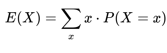
In this problem, there are seven possible values. For the value 0.50, the probability is 4/10. For each of the values 5, 6, 7, 8, 9, 10, the probability is 1/10.
So we have:
Contribution to E(X) from X = 0.50: (0.50) * (4/10) = 0.50 * 0.4 = 0.20
Contribution to E(X) from each of 5, 6, 7, 8, 9, 10: If j is each of these card values, the probability is 1/10, so the sum of these card values is 5 + 6 + 7 + 8 + 9 + 10 = 45. Multiplied by 1/10 each gives 45 * (1/10) = 4.5
Adding these contributions together:
E(X) = 0.20 + 4.5 = 4.70
Hence, the expected payoff is 4.7 dollars.
Second Moment and Variance
To find the standard deviation, we need the variance, which depends on E(X^2). We calculate E(X^2) as follows:
Computing E(X^2)
For X = 0.50, X^2 = 0.25. Probability is 4/10, so the contribution is 0.25 * 4/10 = 0.25 * 0.4 = 0.10.
For X = j in {5, 6, 7, 8, 9, 10}, each j^2 appears once with probability 1/10. So we sum up 5^2 + 6^2 + 7^2 + 8^2 + 9^2 + 10^2: 5^2 = 25, 6^2 = 36, 7^2 = 49, 8^2 = 64, 9^2 = 81, 10^2 = 100. Summing these yields 25 + 36 + 49 + 64 + 81 + 100 = 355. Multiplied by 1/10 each => 355 * (1/10) = 35.5
Hence, E(X^2) = 0.10 + 35.5 = 35.6
Variance and Standard Deviation
The variance of X, denoted Var(X), is:
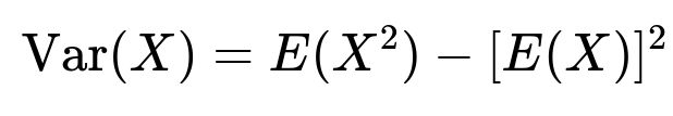
From the calculations:
E(X^2) = 35.6
E(X) = 4.7
So:
Var(X) = 35.6 - (4.7)^2 = 35.6 - 22.09 = 13.51
The standard deviation is the square root of the variance:

Thus:
σ(X) = sqrt(13.51) ≈ 3.68
So the payoff’s expected value is 4.70 dollars, and its standard deviation is approximately 3.68 dollars.
Potential Follow-up Questions
1) Why do we group values 1 to 4 together and assign them the single payoff of 0.50?
When the card is 1, 2, 3, or 4, the game rule says you receive 0.50 dollars (independent of whether it is 1, 2, 3, or 4). That means all these card outcomes lead to the same payoff amount. Hence, we can consider them collectively in a single outcome 0.50 with total probability 4/10.
In probability theory, if multiple events yield the same random variable value, we can aggregate them to simplify the calculation. Instead of enumerating each card from 1 to 4 as separate outcomes with separate probabilities 1/10, 1/10, 1/10, 1/10, we sum their probabilities because they lead to the same payoff.
2) What if we wanted to compute the probability distribution in an explicit tabular format?
You could explicitly list the random variable X’s distribution:
X = 0.50 with probability 0.4
X = 5 with probability 0.1
X = 6 with probability 0.1
X = 7 with probability 0.1
X = 8 with probability 0.1
X = 9 with probability 0.1
X = 10 with probability 0.1
This is a discrete distribution with 7 distinct payoff values. From that distribution, one can compute expectation and variance in the usual manner by summing x * P(X=x) and x^2 * P(X=x) for each x.
3) How might we implement a quick simulation of this game to empirically verify E(X) and std(X)?
Below is a simple Python code snippet that simulates drawing from these 10 cards many times and computes the average payoff and standard deviation empirically:
import random
import statistics

def simulate_game(n_sim=10_000_00):
    payoffs = []
    for _ in range(n_sim):
        card = random.randint(1, 10)  # random card from 1 to 10
        if card < 5:
            payoffs.append(0.50)
        else:
            payoffs.append(float(card))
    return statistics.mean(payoffs), statistics.pstdev(payoffs)

mean_estimate, std_estimate = simulate_game()
print("Estimated Mean:", mean_estimate)
print("Estimated Std Dev:", std_estimate)
In a large enough simulation (e.g. a million draws), these estimates should be close to the theoretical values 4.7 and 3.68.
4) How do we interpret the standard deviation of 3.68 in this context?
The standard deviation measures how much the payoff typically fluctuates from its mean of 4.7 dollars. A standard deviation of about 3.68 indicates that, on average, most payoffs deviate from 4.7 by around 3.68 dollars. Practically, this tells us that while on average you make 4.7 dollars, you can sometimes earn as little as 0.50 (which is well below the mean) or as high as 10, reflecting a relatively wide range of variation for a one-time draw.
5) What would happen if the threshold were different (e.g., you get 0.50 for cards less than 6, or less than 4)?
Altering the threshold changes the probability of each payoff outcome:
If you got 0.50 for cards < 6, then it would be 0.50 for cards 1 to 5, and the actual card value for 6 to 10.
If you got 0.50 for cards < 4, then it would be 0.50 for cards 1 to 3, and the actual card value for 4 to 10.
Each of these scenarios simply changes the distribution of X. The method to compute the expectation and standard deviation remains exactly the same: identify which card values contribute which payoffs, note their probabilities, and then plug these into the formulas for E(X) and E(X^2).
6) Could the result be influenced if the card-draw mechanism had any bias?
Yes. In the real game, if a deck is not truly shuffled or if some mechanical selection process is biased, the probabilities would deviate from 1/10 per card. This would invalidate the assumption that each card is equally likely. The approach to calculating the expected value and standard deviation is the same, but you would have to incorporate the correct probabilities. If a card is more likely to be drawn than another, that outcome’s probability must be adjusted accordingly, and thus the final E(X) and std(X) values would change.
7) What if we repeated the game multiple times and added the payoffs?
If you repeated the game n times independently and summed up all the payoffs, the total payoff random variable Y would simply be X_1 + X_2 + ... + X_n, where each X_i is i.i.d. with the same distribution as X. Then:
E(Y) = n * E(X) = n * 4.7
Var(Y) = n * Var(X) = n * 13.51
Std(Y) = sqrt(n) * 3.68
Such linear properties of expectation and variance are crucial in many real-world applications where repeated independent draws or repeated experiments are performed.
Below are additional follow-up questions
1) How does the distribution’s shape affect higher-order moments like skewness and kurtosis?
In this payoff distribution, the random variable is 0.50 with probability 0.4 and takes the values 5 through 10 each with probability 0.1. This creates an asymmetry where a large chunk of the probability mass is at 0.50, while the rest is spread among higher values 5, 6, 7, 8, 9, and 10.
To compute skewness, for example, you would look at the third central moment (the expected value of (X - E(X))^3) and compare it against the standard deviation cubed. Because so much probability is concentrated at a small value (0.50) while the rest is spread among larger values, the distribution is not symmetric. Intuitively, you expect a right skew (the tail extends to the high-value side). A similar process applies to kurtosis (the fourth central moment).
The pitfall here is assuming a symmetrical distribution and thinking that certain symmetrical distribution properties apply (like mean = median). That is not true for this scenario. You must explicitly calculate or simulate skewness and kurtosis if needed in more advanced analyses.
2) What happens if we introduce negative payoffs for certain cards?
If the game were modified so that drawing certain cards yields a negative payoff (for instance, if you draw card 3, you lose 2 dollars), you would have a payoff distribution that includes values below zero. The general approach to calculating expected value and standard deviation remains exactly the same: each possible outcome multiplied by its probability. But the presence of negatives might reduce the mean, increase the variance, and could shift other properties of the distribution (like skewness).
A real-world pitfall is that negative payoffs imply potential debt or penalty. Some players or analysts might forget to incorporate those negative scenarios carefully, especially when applying certain risk measures. Mistakes can arise if one tries to apply formulas designed for strictly positive payoffs (e.g., some multiplicative utility theories) without adapting them for negative outcomes.
3) How would these calculations change if the card draws are not equally likely?
If the card distribution has unequal probabilities—for instance, if cards 5 through 10 were more likely than cards 1 through 4—then the payoff distribution changes. Let p1, p2, p3, p4 be the probabilities of drawing each of 1, 2, 3, 4, respectively (with each less than 0.1 perhaps), and p5, p6, p7, p8, p9, p10 be those for 5, 6, 7, 8, 9, 10.
The formulas for the expectation and variance would still hold conceptually: E(X) = sum of x * P(X=x) over all x, and Var(X) = sum of x^2 * P(X=x) - (E(X))^2. But now each outcome has its own unique probability. If you do not carefully track these probabilities, you will get incorrect results.
A pitfall in real-life scenarios is assuming equal likelihood when the selection method might be biased (e.g., some mechanical shuffle not truly random). Analysts might hastily apply 1/10 across the board without checking the actual probabilities.
4) Could the standard deviation become zero under any modification of the rules?
Yes, the only way for the standard deviation to be zero is if there is no variability in the random variable, meaning X is always the same value. In this card game context, that would happen if all possible draws resulted in exactly the same payoff. For example, if the game always paid out 0.50 dollars, regardless of the card drawn, then the standard deviation is zero because there is no spread in outcomes.
A subtle pitfall is ignoring small variations in outcomes (like rounding errors or other small differences), which can introduce confusion about whether the distribution is truly constant or just nearly constant. Even a tiny difference in outcomes can result in a non-zero variance, though small.
5) How could we construct a confidence interval for the expected payoff if we only had sample data?
If you do not know the true distribution but instead collect sample payoffs by playing the game multiple times, you can estimate the mean payoff (sample mean) and its sample standard deviation. Then you can form a confidence interval, for example using a normal approximation if the number of samples is large (by the Central Limit Theorem). A typical formula for a 95% confidence interval of the mean payoff might be:
(sample mean) ± 1.96 * (sample standard deviation / sqrt(n))
The main pitfall is that if the sample size n is too small or the distribution is extremely skewed, then the normal approximation might be misleading. In such cases, you might need non-parametric methods (like the bootstrap) to construct more reliable intervals for the mean payoff.
6) What if the cards are drawn without replacement in repeated plays?
Drawing multiple cards without replacement in a single session changes the probabilities dynamically. For instance, if you draw a card and do not put it back, the chance of drawing each remaining card is different in subsequent draws. This violates the assumption of identical independent draws.
To handle this, you must use hypergeometric considerations instead of simple binomial or multinomial logic. The expected value of a single draw still remains the same if you only draw once, but if you consider multiple draws from the same deck without replacement, the distribution of payoffs changes with each draw.
A pitfall is applying formulas for independent identically distributed random variables to a scenario where draws affect each other. That can cause incorrect variance or incorrect probability calculations.
7) How can we apply Markov’s or Chebyshev’s inequality to bound the probability that the payoff exceeds a certain threshold?
Chebyshev’s inequality states that for any random variable X with mean μ and standard deviation σ, the probability that X deviates from μ by more than kσ is at most 1/k^2. So if we want to bound how likely it is that the payoff exceeds, say, μ + kσ, we can use that:
P(X > μ + kσ) ≤ P(|X - μ| > kσ) ≤ 1/k^2
Markov’s inequality can also provide a bound for non-negative random variables X:
P(X ≥ a) ≤ E(X) / a
However, these bounds are often quite loose compared to the actual distribution. A pitfall is relying on these bounds to make precise risk calculations. While they hold in theory for any distribution with a finite mean or variance, in practice they are not always tight enough for real-world risk assessments.
8) If the payoff is piecewise defined, can we interpret it differently for analytical convenience?
Sometimes, you can reframe the game’s payoff distribution in a piecewise manner: for example, define an indicator that checks if the card is less than 5 versus otherwise, and combine that with the numerical value. Mathematically, one might express it as X = (card_value) * I(card_value >= 5) + 0.50 * I(card_value < 5), where I is an indicator function.
This perspective can help if you are integrating with more advanced probability tools or regression modeling. For instance, if you were to treat the card value as a random variable Y from 1 to 10 and then define X = 0.50 if Y < 5 and X = Y if Y >= 5, you could use expectation properties like E(X) = E(0.50 I(Y < 5) + Y I(Y >= 5)). The pitfall is making sure you properly handle each indicator’s domain and do not lose track of conditional probabilities in more complicated setups.
9) Could player strategy influence the outcome if partial knowledge of the deck is revealed?
Imagine a scenario where the player might see or infer something about the distribution of remaining cards before drawing (for instance, if they know some cards have been removed or if there is a partial reveal of certain card positions). In a purely random single draw with no prior knowledge, strategy does not matter. But if partial knowledge is gained—like certain cards are known to be gone—then the probabilities shift for the next draw, and the expected payoff might change.
A pitfall in real games is assuming the original probabilities still hold despite new information (i.e., ignoring Bayesian updates). In a setting where knowledge is gained over time (like counting cards in blackjack), the true distribution at each draw is updated, and thus the expected payoff or standard deviation is no longer the same as the initial calculation.
10) How might practical constraints or real-world conditions alter the game?
In an actual physical card game, there could be accidental reveals, damaged cards, or psychological factors (like how the dealer or player might guess certain positions). There could also be table stakes or maximum payout limits. These real-world factors sometimes invalidate the straightforward assumption of equal probabilities or the exact payoff distribution.
A subtle point is that if there is a rule such as, “If the sum of payoffs in the casino for the day goes above a certain limit, we cap payouts,” that changes the payoff distribution for large draws. Another pitfall is ignoring these caps or misrepresenting them in the model, leading to incorrect estimates of expected payoffs and risk measures.