ML Interview Q Series: Calculating Threshold Exceedances for Normal Samples Using Binomial Probability

Browse all the Probability Interview Questions here.

You have N samples drawn independently from a Normal distribution with mean μ and standard deviation σ. If we set a threshold Y, what is the probability that exactly k of these samples exceed Y?

Comprehensive Explanation

Overview of the Problem

We are dealing with N i.i.d. samples, each drawn from a normal distribution with mean μ and standard deviation σ. We introduce a threshold Y and want the probability that exactly k out of these N samples lie above Y. The key to solving this is:

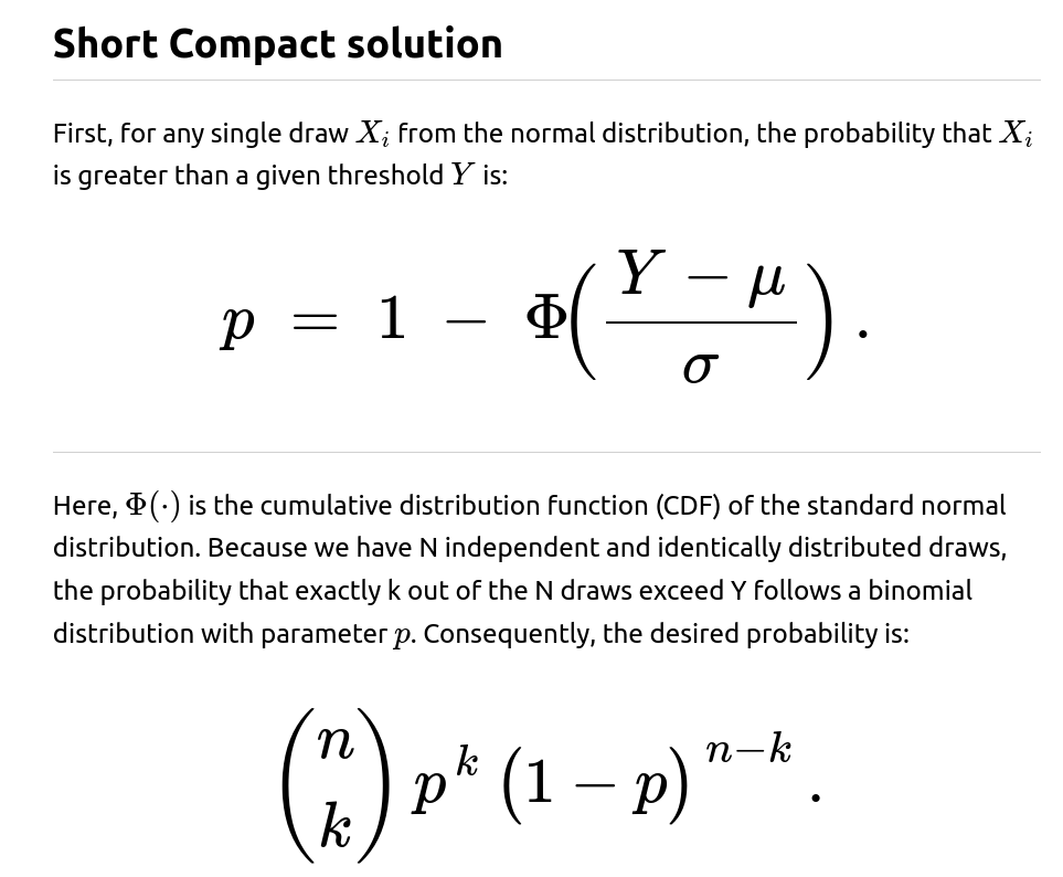
1. Determine the probability of a single draw being above Y.

2. Recognize that counting how many among N draws exceed Y can be modeled as a binomial random variable if the draws are independent.

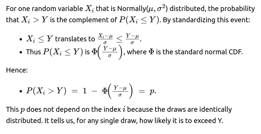
Single-Draw Probability

Binomial Distribution of Counts

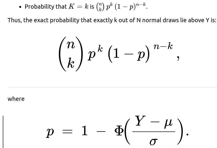
Once we know p, the question “How many out of N exceed Y?” is fundamentally asking about a count of Bernoulli trials. Each draw acts like a Bernoulli trial: “success” if the draw exceeds Y (with probability p), and “failure” otherwise (with probability 1−p). Because these trials are independent, the total count of successes K follows a binomial distribution:

Connection to Real-World Use Cases

In many real-world contexts—such as quality control, anomaly detection, or hypothesis testing—one often checks how many instances exceed a certain specification limit. Under normal assumptions, this approach is straightforward: determine the single-trial exceedance probability p using the normal CDF, then apply binomial reasoning for the count of exceedances.

Implementation Example in Python

Below is an example of how one might quickly compute this in Python. Note that the math.comb function is available in Python 3.8+:

import math
from math import comb
import statistics

def binomial_probability_count_exceeding(n, k, mu, sigma, Y):
    # Single-draw probability of exceeding Y
    from math import erf, sqrt

    # Alternatively, one can use 'statistics.NormalDist().cdf' in Python 3.8+
    # or libraries like scipy.stats.norm for standard Normal CDF.

    # For demonstration: approximate standard normal CDF with erf
    def standard_normal_cdf(z):
        return 0.5 * (1 + erf(z / math.sqrt(2)))

    p = 1.0 - standard_normal_cdf((Y - mu) / sigma)

    # Binomial probability
    return comb(n, k) * (p**k) * ((1 - p)**(n - k))

# Example usage:
n = 10
k = 3
mu = 0.0
sigma = 1.0
Y = 1.5

prob = binomial_probability_count_exceeding(n, k, mu, sigma, Y)
print(f"Probability of exactly {k} out of {n} exceeding {Y}: {prob}")

This code snippet uses a basic approximation for the standard normal CDF. In practice, a more precise function is typically imported from something like scipy.stats.norm.cdf.

Potential Pitfalls

1. Estimation of μ and σ If μ and σ must be estimated from data rather than being known a priori, there is an additional source of uncertainty. One might then use a plug-in approach (simply replace μ and σ with their estimates) or adopt a Bayesian approach to model the posterior distribution of μ and σ and integrate out that uncertainty.

2. Large N Approximations For very large N, the binomial distribution can be approximated by a normal distribution or a Poisson distribution (depending on the size of p). However, if p is not extremely small or extremely close to 1, the normal approximation with mean np and variance np(1−p) is the more common approach.

3. Edge Cases

   • If p is extremely close to 0 or 1, numerical underflow or floating-point inaccuracies might occur in direct binomial computations. Use log probabilities or specialized libraries for stability.

   • If k=0 or k=n, handle corner cases carefully but the binomial formula still holds.

4. Non-Normal Distributions If the samples do not come from a normal distribution, the single-draw probability might be estimated differently, and the result might still form a binomial distribution if the draws are i.i.d. However, p would be computed from the correct distribution’s CDF.

5. Correlated Draws If the N draws are not independent, the count of exceeding Y would not strictly follow a binomial. Approaches in such scenarios could involve modeling the correlation structure (e.g., using copulas or other correlated distribution assumptions).

Follow-Up Questions

1) What if the mean μ and standard deviation σ are not known?

In many practical situations, μ and σ might be unknown and need to be estimated from data. One straightforward approach is:

However, this introduces estimation error. If the sample size is large, the plug-in estimates work reasonably well. In more advanced methods, one might:

• Use a Bayesian framework with priors on μ and σ, then integrate over their posterior.

• Use bootstrap techniques to quantify the variability in the estimate of p.

2) Why does this scenario boil down to a binomial distribution?

A binomial distribution arises whenever we have N independent Bernoulli trials, each with the same probability p of “success.” In this context:

• Each draw is a Bernoulli trial because it either exceeds Y (success) or not (failure).

• The probability of success is identical for all draws (p), assuming identical distribution and independence.

Hence, the count of successes is binomial by definition. If draws were correlated, or did not share the same p, we could not strictly rely on the binomial distribution.

3) Could we use a normal approximation instead of a binomial?

For large N, the distribution of K (the number of successes) can be approximated by a normal distribution with mean np and variance np(1−p). Specifically:

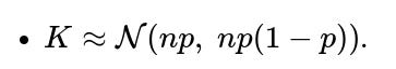
However, the accuracy of this approximation depends on how large N is and whether p is away from extreme values (close to 0 or 1). A common guideline is that both np and n(1−p) should be larger than some constant (often 5 or 10) to achieve a decent approximation.

4) How can this be extended to the probability that at least k samples exceed Y?

To find the probability that at least k samples exceed Y, we sum over the relevant binomial probabilities:

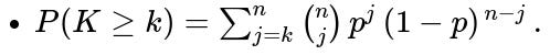
In code, one might loop from j = k to n, or make use of cumulative distribution functions for the binomial, which are readily available in libraries like scipy.stats.

5) How do we address numerical issues for large n?

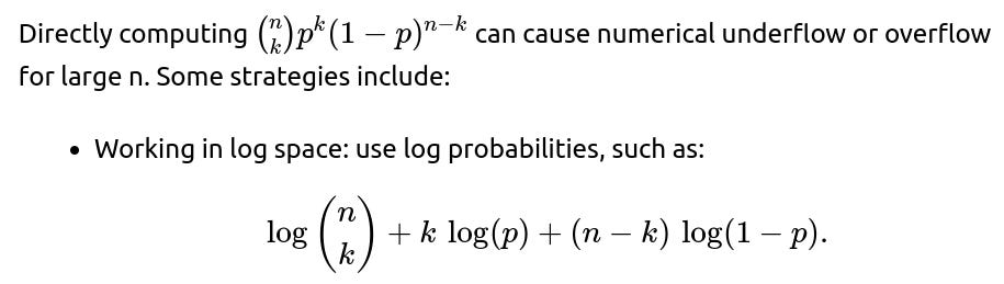
• Then exponentiate at the end if needed.

• Using specialized libraries (e.g., scipy.special.comb in Python with exact or floating support, and scipy.stats.binom for binomial probabilities).

6) How do we implement this if we must do it repeatedly for different values of Y?

If we need to evaluate different thresholds Y in rapid succession, we can:

• Compute the normal CDF values ahead of time (e.g., a table or interpolation for Φ).

• Reuse partial computations when n and k remain fixed but Y changes.

For large-scale or real-time systems, vectorized computations in libraries like NumPy/SciPy or GPU-accelerated approaches can be used to handle many thresholds at once.

Below are additional follow-up questions

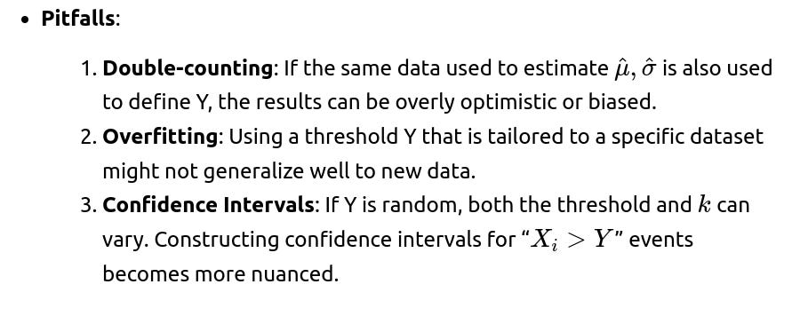
1) What happens if the threshold Y itself is random or learned from the data?

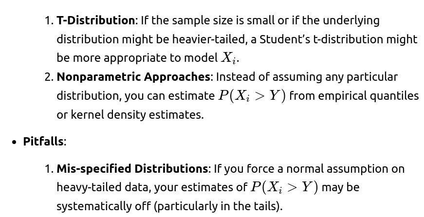
2) How do we proceed if the normal distribution assumption does not hold?

When the data does not follow a normal distribution, the probability of exceeding Y must be derived from the actual data distribution or alternative assumptions.

Detailed Explanation

• Alternative Distributions:

  

  2. Data Scarcity: Nonparametric methods can fail if you do not have enough data to robustly estimate the tail or the distribution near Y.

• Practical Steps:

  1. Use Goodness-of-Fit Tests: Check whether your data truly looks Gaussian (e.g., with Q-Q plots or statistical tests).

  2. Compare with Empirical: Compare your theoretical p with an empirical fraction from historical data or a hold-out set to see if the assumptions align.

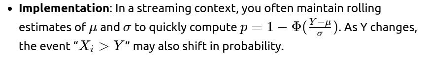
  3) Could the threshold Y change over time or in a streaming environment?

  Yes. In real-time or streaming scenarios, thresholds might be dynamic, adjusting as new data arrives.

  Detailed Explanation

  • Dynamic Threshold: If Y is updated periodically (e.g., monthly) based on recent data distributions or business requirements, the value of p can shift over time.

    

    Pitfalls:

    1. Concept Drift: If μ or σ is not stationary—maybe the process evolves—the distribution changes, and older estimates of p or Y become outdated.

    2. Lag in Updating: If you delay the update of Y or the parameters, you might produce incorrect short-term predictions.

    3. Computational Constraints: Continuously updating distribution estimates and the threshold in real time can be computationally expensive. You may need approximate methods or incremental algorithms (like Welford’s online algorithm for mean and variance).

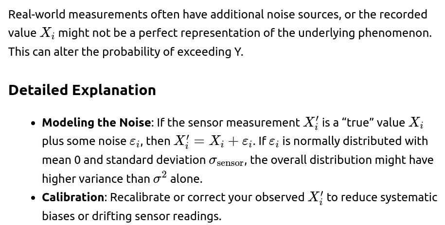
4) In practice, how can we account for measurement noise or sensor errors?

• Pitfalls:

  1. Unaccounted Extra Variance: If the sensor noise is substantial and you do not incorporate it, your probability p of exceeding Y may be inaccurately computed.

  2. Unrecognized Bias: A sensor might consistently overread or underread, shifting the measured distribution’s mean.

  3. Uncertainty Propagation: In some advanced methods, you explicitly model sensor uncertainty so that your final exceedance probability includes that additional variance.

     5) What if the number of draws N is itself random?

     Sometimes, N is not a fixed value but random—e.g., if data is collected until a resource limit is reached or a stopping criterion is met.

     Detailed Explanation

     • Two-Stage Randomness: Now there is randomness in both how many samples you collect and how many exceed the threshold. You would need the distribution of N (e.g., Poisson, negative binomial, or any other discrete distribution) to proceed.

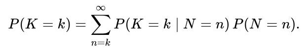
     • Compound Distribution: The probability that K=k can become a mixture over all possible values of N. For instance, if N is Poisson with mean λ, then:

       

       Pitfalls:

       1. Complex Modeling: Summing or integrating over the distribution of N is more complex and might involve infinite sums.

       2. Approximation: For large or indefinite N, you might rely on approximations (e.g., normal approximations or bounding techniques).

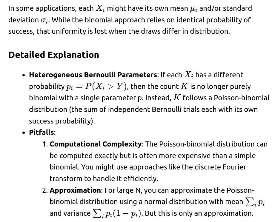
     6) How does this binomial approach change if the draws have different means or standard deviations?

     

     7) Can we combine this procedure with other statistical tests?

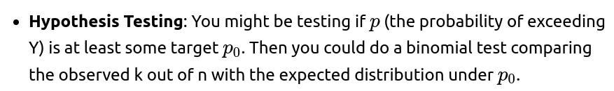
     Sometimes, we are not just interested in the count of exceedances but also in how that count relates to an underlying hypothesis or a performance threshold.

     Detailed Explanation

     

     Confidence Intervals: Alternatively, you can construct a confidence interval for p from the binomial distribution. For instance, using a Clopper-Pearson interval or a Wilson interval might be more stable for smaller sample sizes.

     Pitfalls:

     1. Multiple Testing: If you are repeatedly testing with different thresholds Y, you might inflate your Type I error rate unless you adjust for multiplicity.

     2. Assumption of Independence: If the draws are correlated, standard binomial tests are invalid. You may need a block-resampling method or a generalized linear mixed model to account for correlations.

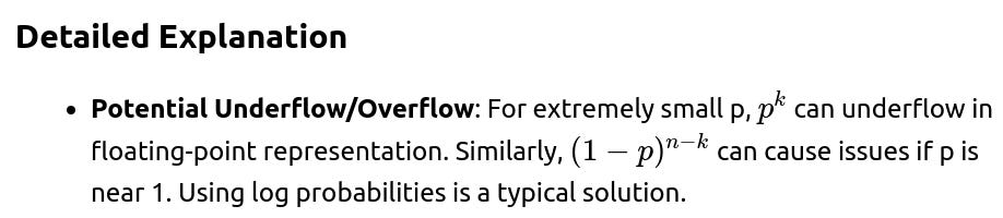
  8) How might we handle very extreme thresholds where p is extremely small or extremely large?

  When p is near 0 or 1, numerical instabilities and interpretive difficulties arise.

  

  Interpretation: If p is extremely small, seeing even a single exceedance might be highly significant. Conversely, if p is extremely large (close to 1), not exceeding Y even once could be surprising.

• Pitfalls:

  1. Poor Approximation by Normal: The normal approximation to the binomial might be very inaccurate for extreme p.

  2. Sparse Observations: If p is extremely small and the phenomenon is very rare, you might not have enough data to confidently estimate p (the zero-inflation problem).

9) Is there a scenario where the draws might become conditionally dependent after observing some are above Y?

Yes. If subsequent draws or the threshold Y adapts based on whether earlier draws exceeded Y, you lose independence.

Detailed Explanation

• Sequential Adaptive Trials: In A/B testing, for instance, if you see enough “successes” or “failures,” you might stop the test early or change the threshold. This adaptive design leads to correlated data.

• Bayesian Updating: If you are updating your belief about μ and σ online and also adjusting Y, then each new draw influences the next threshold, introducing a correlation that breaks the simple binomial form.

• Pitfalls:

  1. False Assumption: Treating these draws as i.i.d. can yield biased results.

  2. Advanced Methods: You might need specialized sequential analysis methods (e.g., Thompson sampling in multi-armed bandits) or fully Bayesian approaches that explicitly model the entire process.

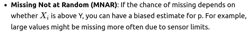
10) How does one handle missing data among the N draws?

In real-world data collection, some of the N observations might be missing or unreliable.

Detailed Explanation

• Missing Completely at Random (MCAR): If the data is missing randomly and not biased by the actual values, you can reduce N accordingly and still apply binomial logic to the subset that remains.

  

  Pitfalls:

  1. Bias: Excluding missing data without adjusting can lead to incorrect estimates of how many draws truly exceed Y.

  2. Multiple Imputation: One might consider statistical imputation or bounding methods (e.g., worst-case vs best-case) to see how robust the result is when some draws are missing.