
ML Interview Q Series: Calculating Median Probability for Uniform Samples Using Binomial Logic

Browse all the Probability Interview Questions here.
Suppose you take three independent random samples from a uniform distribution on the interval (0, 2). What is the probability that the median of these three samples exceeds 1.5?
Short Compact solution
Because the median of three values is the one in the middle, it will be at least 1.5 if and only if at most one of the three values is strictly below 1.5 (the other two must then be larger than 1.5). Each draw has a probability of 3/4 of being less than 1.5 (since 1.5 is 3/4 of the way along the interval from 0 to 2). We then calculate the probability that at most one out of the three samples is below 1.5. This is the sum of the probabilities that exactly one sample is below 1.5 plus the probability that none are below 1.5. That sum is

Hence, the final probability is 5/32.
Comprehensive Explanation
Overview
We want the probability that the median of three uniformly drawn samples from 0 to 2 exceeds 1.5. The median is the second-largest (or second-smallest) among the three values once they are sorted.
To approach this, it helps to break down what it means for the median to be above 1.5:
If the median is to exceed 1.5, we can allow at most one of the three samples to be below 1.5.
Equivalently, if two or more samples were below 1.5, the median would be below or equal to 1.5.
Probability of a Single Draw Being Below 1.5
Because each draw is from a Uniform(0, 2) distribution, we compute:
Interval length is 2.
The threshold of interest is 1.5.
So the probability that a single sample is below 1.5 is 1.5 / 2 = 3/4.
Consequently, the probability that a single sample is 1.5 or above is 1 - 3/4 = 1/4.
Counting Valid Configurations
We want “at most one sample below 1.5.” That splits into two disjoint scenarios:
Exactly one sample below 1.5.
First choose which one of the three samples is below 1.5: there are 3 ways to choose which sample is the "below 1.5" draw.
Probability that chosen sample is indeed below 1.5: 3/4.
Probability that the other two samples are 1.5 or above: (1/4) each.
Combine these: 3 × (3/4) × (1/4)².
No samples below 1.5.
All three samples are 1.5 or above.
Probability: (1/4)³.
Add them up to find the total probability:

Hence, the median exceeds 1.5 with probability 5/32.
Intuitive Reasoning
The uniform distribution between 0 and 2 means any value in that interval is equally likely. For the median to be on the higher side (above 1.5), it essentially means “most of the values have to be on the higher side.” Since 1.5 is 3/4 of the interval, there is a 3/4 chance for a sample to be below 1.5, but we can only afford at most one such occurrence in the three draws for the median to remain above 1.5. Counting those configurations carefully yields 5/32.
What If Interviewers Ask More?
Below are several deeper follow-up questions that interviewers might pose, each followed by a thorough discussion.
If the distribution were not uniform, how would we approach this?
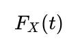
If the distribution was not uniform, you would need to know the cumulative distribution function (CDF). Suppose the random variable has a CDF

. Then the probability of a single draw being less than a threshold t is

. To get the probability that the median is above t, you again require at most one draw to be below t. The general approach remains:
Probability a single draw is below t is
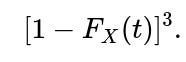
2. Probability a single draw is at least t is 1 −

3. At most one draw below t can happen in exactly 0-below-t or 1-below-t scenarios. So you would sum:
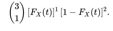
Probability(exactly one below t) =

Probability(none below t) =
Add them to get the final probability.
Even though the integral expression for non-uniform distributions can be more involved, you can still tackle it by carefully enumerating or by integration (if you prefer a direct approach using the joint density of three samples).


How would this generalize to n samples instead of 3?
For n samples, the median is the

th order statistic when n is odd. Suppose we want the probability that the median is greater than some threshold t. We then require that fewer than half of the samples lie below t. For an odd n = 2k+1, the median is the (k+1)-th largest, meaning at least k+1 samples must be ≥ t. That is equivalent to at most k samples below t. Therefore, the probability is:

With a uniform(0, 2) distribution and threshold t, you substitute F_X(t) = t/2 for the relevant t in the interval [0,2].
Could we have solved it using integrals directly over the joint PDF?
Yes. Another approach is to integrate the joint density of three i.i.d. random variables over the region in which the median is greater than 1.5. Specifically, the joint PDF for three uniform(0,2) variables X1, X2, X3 is:

You would then integrate over the set of (x1, x2, x3) such that at most one xi is < 1.5:

Although straightforward, it can be tedious. You partition the integration space into disjoint events: (0 are below 1.5) + (1 is below 1.5). Each region is easier to integrate separately. Once done, you get the same 5/32 result.
Why is the calculation using “strictly greater” or “greater or equal” not changing the result?
Because the distribution is continuous, the difference between “> 1.5” and “≥ 1.5” is a set of measure zero, which does not affect probabilities. In discrete distributions, that difference would matter, but not for a continuous uniform distribution.
What are some potential edge cases?
If the threshold were 0 or 2, the probability might trivially be 1 or 0. But for an interior point like 1.5, we do a proper binomial-based or integral-based approach.
If the distribution had heavier tails or a domain that did not include 1.5, then the probability would be 0 or 1 accordingly.
With degenerate distributions (like a random variable that is always 1.7), the “median above 1.5” probability would obviously be 1, and none of the usual binomial or integral approaches would be interesting.
How can I simulate this in code?
Below is a simple Python snippet that runs a Monte Carlo simulation to empirically estimate the probability. This is often used as a sanity check:
import numpy as np

N = 10_000_000  # number of trials in the simulation
samples = np.random.uniform(0, 2, (N, 3))
medians = np.median(samples, axis=1)
prob_estimate = np.mean(medians > 1.5)
print(prob_estimate)
If you run this, you should see a value close to 0.15625 (which is 5/32) as N grows large.
All these variations—analytical and computational—consistently confirm that the answer for a uniform(0,2) distribution is 5/32.
Below are additional follow-up questions
What if the random draws are not independent?
In the original problem, each draw is assumed to be an independent uniform(0,2) random variable. However, suppose there is some correlation between draws. For instance, if you have a hidden factor that causes the draws to be simultaneously higher or lower than average. In such cases:
Impact on Probability: The event “median exceeds 1.5” is no longer a straightforward binomial-style computation. If two samples are correlated to move together, it might be more likely (or less likely) that they both exceed 1.5 at the same time, altering the probability.
Modeling the Dependence: You would need to specify or estimate the joint distribution of the three samples. A common approach might be using a multivariate distribution, such as a multivariate Gaussian restricted to the interval (0,2), or a copula-based model if you only know correlation structures.
Pitfall: If one tries to compute the probability by simply plugging in the marginal probabilities (i.e., “3/4 for being below 1.5”), ignoring correlation, one might arrive at an incorrect answer. Joint distributions must be used to capture the dependence structure accurately.
In practice, you would integrate or sum over the joint probability density function that describes all three draws together. The final result could differ significantly from 5/32, depending on whether correlation makes the samples cluster above or below 1.5.
What if there are outliers or extreme values in real-world data?
While a uniform(0,2) distribution is simple, real-world data may have heavy tails, spikes, or “outliers.” Outliers can affect the ranking of observations if they occur in the lower or higher range:
Median’s Robustness: The median is more robust to outliers than the mean, so a single extreme value may not hugely change whether the median is above 1.5. However, two large outliers could shift the median higher, and two small outliers could shift it lower.
Data Transformations: Analysts sometimes log-transform data (especially if it spans several orders of magnitude) to reduce the impact of extreme observations. This changes the distribution shape and modifies how you’d interpret “above 1.5” on the transformed scale.
Pitfalls: If you assume uniformity without checking real data distribution, your probability estimate may be off. Non-uniform distributions with heavier tails can concentrate samples differently around 1.5, shifting that probability.
In an interview, you might be asked to highlight that the simplistic result of 5/32 relies on an idealized assumption that the distribution is truly uniform with no outliers.
Could the median be exactly 1.5 with nonzero probability for a continuous distribution?
In a continuous distribution like uniform(0,2), the probability of any single sample exactly equaling 1.5 is zero because there is an uncountably infinite set of possible values. Consequently:
Probability of Exact Equality: The measure of the point x = 1.5 is zero, so the chance that a draw lands exactly there is zero.
Median’s Exact Value: For three independent continuous draws, the event “median equals 1.5 exactly” has measure zero as well.
Practical Implications: When computing the probability of the median exceeding 1.5 vs. being at least 1.5, both events have essentially the same probability. In real data with measurement precision, 1.5 might appear more often because of rounding, but theoretically the probability remains negligible under truly continuous assumptions.
Hence, in interviews or theoretical discussions, it is important to emphasize that “≥” and “>” are essentially the same in continuous distributions.
How do we handle discrete distributions?
If instead of a continuous uniform distribution, the random variable takes values from a discrete set (like {0, 1, 2} with certain probabilities), the reasoning about the median changes:
Non-zero Probability at Single Points: Discrete distributions can assign non-zero probability to individual points. In that scenario, the probability the median equals exactly 1.5 may be nonzero only if 1.5 is in the support. If 1.5 is not a supported value, the median might jump between 1 and 2, or other discrete points.
Order Statistics in Discrete Case: To find the probability the median is above a specific cutoff, you’d sum over all combinations in which at least two of the draws exceed that cutoff. The combinatorial approach remains valid, but the probabilities p = P(X < 1.5) and 1 - p might not be as straightforward as 3/4 or 1/4. You must use the actual pmf (probability mass function) to get these values.
Edge Cases: Discrete distributions can have abrupt changes in probability. Even a small shift in the cutoff can drastically alter the probability if the cutoff crosses a major jump in the pmf.
Overall, you need to carefully account for the discrete probability mass at and around the cutoff rather than applying continuous logic directly.
What if the random variable’s range is not [0, 2] in practice?
If real-world data extends beyond 2, or perhaps doesn’t start at 0, the original problem statement might not hold:
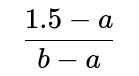
Different Support: Say the real data is uniform on (a, b) for some a and b. Then the fraction of the interval up to 1.5 is

if 1.5 lies between a and b. If 1.5 < a or 1.5 > b, the probability that the median exceeds 1.5 could be trivial (either 0 or 1).
Handling Shifts or Scales: If the dataset is uniform on (0, K) for some K ≠ 2, you can still do a direct ratio

if 1.5 ≤ K to find the probability below 1.5. The same binomial logic works: at most one draw can be below 1.5.
Potential Pitfall: A common mistake is to blindly reuse 3/4 for the probability a draw is below 1.5, even though the distribution might no longer be uniform(0,2). It is critical to recalculate that probability for the new domain.

In an interview, you might be asked to adapt your solution quickly when the domain changes, to show your ability to generalize the approach to any (a, b).
How can a bootstrap approach be used to estimate or confirm this probability from sample data?
In real datasets where the distribution is unknown but we do have a sample dataset:
Bootstrap Steps:
Draw a large number of bootstrap samples by sampling with replacement from the observed dataset.
For each bootstrap sample of size N (in this case 3 if you’re mimicking the original scenario, or more if you want to approximate the overall distribution better), compute the median and check if it exceeds 1.5.
Estimate the probability as the fraction of bootstrap samples whose median is above 1.5.
Why Useful: This method does not require knowing the underlying distribution. It relies only on the assumption that your observed dataset is representative of the true data-generating process.
Pitfalls: If the sample data is small or unrepresentative (for example, if your dataset does not capture the true variability or has selection bias), the bootstrap estimate may be off. You must be cautious about the independence assumptions in your data.
This question can test your familiarity with nonparametric methods for probability estimation, which is valuable in cases where analytic solutions are not easily derived.
What if there is partial knowledge or truncated observations in real-world scenarios?
Sometimes you only know that values lie above or below certain thresholds, or some data is missing:
Truncation: For example, you might only observe X if it is ≥ 0.7. This changes the effective distribution for each draw. The correct approach is to use the conditional distribution on [0.7, 2].
Censoring: If you only know that a given draw is below 0.5 but not exactly how much below 0.5, you again have to account for the partial information. The distribution you use to compute the probability that the median is > 1.5 needs to reflect this censoring.
Pitfalls: If you ignore truncation or censoring, your probability estimates can be badly biased. Correct methods might require maximum likelihood with censored data or survival analysis techniques.
Interviewer Expectation: They may check if you realize that real-world data frequently has incomplete observations, and you must adapt the probability assessment using the truncated or censored likelihood framework.