ML Interview Q Series: Calculating SaaS LTV: Churn Rate Models vs. Observed Customer Lifespan Data.

Browse all the Probability Interview Questions here.

Suppose you are working at a SaaS company that has been operating for just over twelve months. The Chief Revenue Officer requests the average LTV (lifetime value). The service is priced at $100 per month, there is an approximate 10% monthly churn, and customers usually stay subscribed for around 3.5 months. What would be the formula to determine the average lifetime value?

Comprehensive Explanation

A common way to model Lifetime Value (LTV) in a subscription-based setting is to connect the revenue per month (or average revenue per user, ARPU) with churn (i.e., the percentage of subscribers who drop the service each month). One canonical formula relies on the assumption of a constant monthly churn rate and uses the reciprocal of churn to estimate average customer lifespan. However, the problem here states both a specific churn rate (10%) and a measured average subscription length (3.5 months). This can lead to different numerical outcomes depending on the assumptions made.

Core Formula for LTV Under Constant Churn Model

When a business treats churn as a constant fraction of customers leaving each month (often approximating an exponential decay), a well-known formula for LTV (neglecting discount rates) is:

If we denote monthly churn by c (for instance, c = 0.1 for 10% per month), and the monthly subscription cost (or revenue) by m, then the average lifetime of a customer (in months) under this idealized assumption is 1/c. Hence:

• Monthly revenue per user = m

• Churn rate = c

• Average lifespan in months = 1/c

• LTV = m * (1/c) = m / c

In the scenario of a 10% monthly churn (c = 0.1) and a monthly price m = 100, this formula would give:

• Average lifespan of 1/0.1 = 10 months

• LTV = 100 / 0.1 = 1000

Reconciling the 3.5 Months Observation

However, the problem statement explicitly indicates that the observed average duration for customers is about 3.5 months, which is a shorter span than the 10 months one would predict with a straightforward constant churn model. This discrepancy can arise from various practical considerations:

• Business still in early phases: The company has existed only for a little over a year. Observed data may reflect partial customer lifespans and might not mirror the long-term stable churn pattern.

• Heterogeneous cohorts: Different user cohorts (users who joined in different time windows) might have different churn behaviors, making a single “10% churn” not fully accurate across all cohorts.

• Inconsistent churn measurement: The 10% churn figure might be an aggregate, or it might be projected rather than precisely measured, leading to a mismatch with actual retention.

If the company trusts its measured “around 3.5 months” figure as the true average length of stay, then a more direct formula for LTV becomes:

Plugging in the numbers, that would be 100 * 3.5 = 350. In that event, the average LTV is 350.

Choosing the Right Formula

Both expressions are valid for specific assumptions:

1. LTV = monthly_revenue / churn is accurate for an exponential survival assumption and a stable churn rate over a sufficiently long period. It often serves as a theoretical or long-term yardstick.

2. LTV = monthly_revenue * observed_lifespan is a simpler, more direct calculation from empirical data but may miss longer-term dynamics if the company is new and has not observed full lifecycles for all its customers.

Many organizations start by using the second approach (monthly revenue * observed average duration) to get a quick, real-world snapshot, and gradually adopt a more sophisticated model (the 1/churn approach) as they gather more robust churn data and see stable patterns of user retention.

Possible Follow-up Questions

Could you explain why 10% monthly churn usually implies an average subscription of 10 months, but the data shows 3.5 months?

Constant churn at 10% per month in a textbook scenario suggests each month 10% of remaining customers leave, so the expected remaining fraction of any cohort shrinks exponentially. This translates to an average of 1/0.1 = 10 months before a user churns out. However, when real data indicates 3.5 months, it suggests that at this early stage (only a year of operation), churn or retention patterns might deviate from the perfect exponential model. Perhaps new customers who joined only recently have not had enough time to display extended stay patterns, or the churn rate measured over short windows (or across different cohorts) is not stable. Real-world churn can vary drastically depending on customer fit, marketing channels, or product maturity, so a simpler direct observation (3.5 months) can temporarily dominate until more data is collected.

How would you factor discounting or the time value of money into LTV calculations?

In many practical settings, money you receive today is worth more than money you receive a year from now. Thus, you would apply a discount factor d (often representing annual or monthly discount rates) to future revenues. A simple approach might replace the raw sum of monthly payments with a discounted sum. In the constant churn model without expansions or upsells, the discounted LTV formula can become:

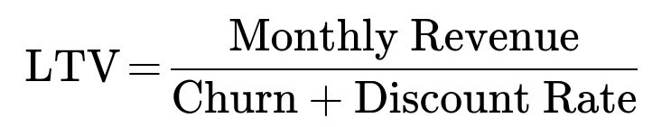
For example, if your monthly discount rate is 0.01 (1% monthly) and your churn rate is 0.10 (10% monthly), then the denominator becomes 0.11. This reduces your LTV relative to the no-discount scenario.

What happens if there are multiple subscription tiers or discount plans?

When multiple subscription tiers exist, each with different monthly pricing and potentially different churn patterns, you can calculate a weighted average LTV across tiers or compute an LTV for each tier separately. For example:

• Tier A: $50/month, churn 8%

• Tier B: $100/month, churn 10%

• Tier C: $200/month, churn 15%

You would produce distinct LTV values for each tier, or you could aggregate them weighted by the fraction of customers who belong to each group. Cohort analysis is often extremely helpful, segmenting LTV calculations by customer type, acquisition channel, or subscription plan.

How would you modify LTV if your product sees “negative churn” due to upsells or expansions?

Negative churn means existing users, on average, upgrade or expand their usage such that the total monthly revenue from the retained users actually grows over time. If you track the net revenue retention rate (factoring both downgrades and expansions) as r, you can embed that into the LTV formula, often yielding a higher LTV because expansions offset the pure loss from churn. A simplified approach might replace “churn” in the denominator with an effective rate that includes expansions. For example, if the expansions from retained customers effectively add 5% additional revenue monthly, your net churn might be 10% - 5% = 5%, which would double the LTV relative to a pure 10% churn with no expansions.

How do you handle acquisition costs (CAC) in LTV calculations?

LTV on its own typically reflects only the gross revenue from a single customer over their lifetime. In many financial metrics, companies want to look at LTV - CAC (Customer Acquisition Cost). If it costs you 200 in marketing to acquire a user, and the LTV is 350, you have 150 net contribution from that user (ignoring operational costs). If your LTV is 1000, you have 800 net contribution after covering the 200 acquisition cost. This difference is crucial for deciding how aggressively to invest in marketing and sales.

Are there any hidden assumptions that can make the simple LTV calculations misleading?

Several underlying assumptions can lead to confusion:

• Constant churn: Real churn may vary by cohort, user demographic, or usage intensity.

• No reactivation: Often, some portion of churned users might return in the future, which is ignored in basic LTV models.

• No discounting: In many real-world analyses, you do want to discount future cash flows.

• No additional revenue: Some businesses offer expansions, upsells, or cross-sells that can alter the basic formula.

A rigorous approach typically involves modeling user survival rates over time (possibly with survival analysis techniques) and tracking expansions/downgrades across cohorts, ensuring the numbers reflect true behavior in the user base rather than idealized assumptions.

Below are additional follow-up questions

How would you handle usage-based or consumption-based pricing models when calculating LTV?

In many modern SaaS platforms, revenue is not strictly tied to a fixed monthly subscription but may depend on how much the customer consumes—for example, a platform that charges per API call, per gigabyte of storage, or per active user seat. In these scenarios, monthly revenue can fluctuate significantly for each customer.

One approach is to segment customers based on average monthly consumption. You might track each customer’s average usage across a given window (e.g., the last three months) and then look at churn and revenue patterns for each usage level. For instance, high-usage customers might churn at a different rate (possibly lower because they derive more value from the product), while low-usage customers may churn more frequently.

A potential pitfall is mixing together customers with wildly different usage patterns into one single LTV calculation. This can lead to a distorted view of average LTV, especially if a few high-usage customers dominate total revenue. Instead, you often do a cohort-based or segment-based LTV approach, ensuring each segment’s churn and revenue data is correctly accounted for. Machine learning models can then be used to predict each customer’s expected usage over time, and that predicted usage profile becomes part of the LTV calculation.

What if there are seasonal or cyclical patterns in churn and revenue?

Many businesses see churn rates and usage fluctuate over seasons—for instance, an education-focused SaaS might see spikes at the beginning of a school term and troughs during vacation. In that case, a single monthly churn figure might be misleading if it is averaged across highly variable seasonal months.

A deeper approach is to model churn on a monthly or quarterly basis, factoring in seasonality explicitly. You might observe that churn is only 5% during certain high-demand months, but spikes to 15% during lower-demand months. One subtle edge case is that an annual subscription might renew in the same month each year, creating cyclical revenue retention that skews the monthly churn measure. If you do not disentangle these effects, LTV calculations can be off by a large margin.

You could employ time-series analysis or advanced forecasting methods. Some organizations prefer rolling cohorts, analyzing how customers who joined during a specific time behave through each subsequent season. By comparing multiple cohorts across multiple seasons, you get a clearer sense of the “true” average churn pattern.

How do you account for partial churn, such as reducing the number of seats or downgrading plan tiers?

Some SaaS platforms allow customers to reduce seats (for instance, going from 100 seats to 70 seats) or downgrade from a premium plan to a standard plan. These partial churn scenarios do not show up in the same way as a total cancellation. Instead, monthly revenue from that account drops without the account fully leaving.

One approach is to define “gross churn” and “net churn.” Gross churn captures the total revenue lost from full cancellations plus any plan downgrades. Net churn offsets that gross churn with any expansions or plan upgrades within existing accounts. LTV becomes more realistic if it’s based on net churn, especially in enterprise SaaS where expansions can be significant. However, at an account level, you can track seat-level changes or plan-level changes in a more granular forecast model. A potential pitfall here is double-counting expansions or ignoring partial downgrades that eventually lead to full churn, so you want to keep rigorous data on how seat counts or plan types evolve each billing cycle.

How do free trials, partial-month subscriptions, or promotional discounts affect LTV?

Free trials can affect both the measured churn rate and the overall LTV because users who abandon the product during or right after the trial might be counted as churn without ever contributing revenue. If your metrics are not carefully segmented between trial users and paying users, your measured churn might look artificially high, and your LTV might look artificially low.

Additionally, partial-month subscriptions or promotional discounts (for example, the first three months are 50% off) can blur monthly revenue calculations. Some companies choose to normalize or annualize revenue to avoid confusion (e.g., compute an annual contract value, or ACV). Others will keep separate segments: one for the trial/promotion period and one for post-promotion revenue. A key pitfall is blending all revenue streams together without considering the proportion of customers still in promotional phases versus those paying the standard rate.

How do you handle incomplete or missing data in an LTV calculation?

In early-stage startups or systems with incomplete tracking, you might have partial records of revenue or churn. This can arise when migrating to a new billing system or from inconsistent logging. If the data is missing in a non-random way, it can bias the LTV estimate.

You can use imputation methods or restrict your analysis to cohorts where you have full revenue and churn data. Another tactic is to combine external data, such as payment logs or CRM exports, to patch missing elements. A subtle trap is to assume that missing data is random when it might be correlated with churn—customers who churned might have incomplete usage data because they left abruptly, meaning your recorded usage logs do not reflect their final usage patterns. In such cases, a more sophisticated survival analysis approach with censored data might be necessary to avoid bias.

Could a machine learning model help predict LTV more accurately?

A machine learning approach can be employed to predict churn or user lifetime based on historical usage features, demographic variables, customer engagement metrics, and so on. Instead of relying on a single monthly churn estimate, you might build a model that estimates the probability a user will churn in each upcoming month. Summing the expected revenues across all months yields a predictive LTV at the individual user level.

However, building such a model has potential pitfalls:

• Data leakage: Using post-churn data points to predict churn can artificially inflate model performance.

• Concept drift: User behaviors and product features can change over time, invalidating an older model.

• Complex calibration: Models might be well-calibrated for one user segment but poorly calibrated for another.

In practice, you typically ensure your data is segmented by cohort, you carefully define features only available at the time of prediction, and you retrain or recalibrate your model periodically to keep up with product changes and user behaviors.

What if our churn rate is not constant but instead changes substantially with user age?

Often, new users have a higher churn risk in the first few months (onboarding or “honeymoon” period). Users who survive that initial period might then exhibit a lower churn rate. Alternatively, in some products, engagement might drop over time. A single churn number (like 10% monthly) can obscure this dynamic.

You can model churn as a function of “user age” or “time since signup,” sometimes referred to as a hazard function in survival analysis. One way is to use a survival function S(t), which estimates the probability that a user remains active at month t. If you integrate over S(t) times the monthly revenue, you get a more nuanced LTV:

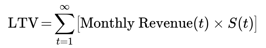
where S(t) is the probability a user is still active at month t, and Monthly Revenue(t) might change over the user’s lifetime due to expansions or discounts. This approach requires sufficient data to fit or estimate S(t). A pitfall is insufficient historical data to confidently model long-term survival, especially if your product is relatively new. Even small errors in the survival function early on can propagate into large LTV miscalculations.

In what ways can an overly simplistic LTV metric lead to poor strategic decisions?

An oversimplified LTV model might ignore real-world complexities like partial churn, seasonality, product-led growth, or expansions. Managers might rely on a single average LTV figure to make decisions on marketing spend or customer acquisition channels. If the LTV number is inflated (for instance, by ignoring discounting or ignoring higher churn in early user cohorts), the company might overspend on ads or promotions under the assumption of profitability that never materializes.

Conversely, if the LTV estimate is too low because expansions and upsells were not accounted for, the company might under-invest in acquiring potentially high-value customers. Another common mistake is ignoring cost structure. Even if the gross LTV is high, net contribution might be small or negative once you factor in operational costs beyond acquisition, such as infrastructure, support, or partner commissions.

What are some specific pitfalls when applying the “1 / churn” rule blindly?

1. Mismatch with actual data: If you measure monthly churn at 10% but real user data shows an average lifetime of only 3.5 months, then 1 / 0.1 = 10 months is misleading.

2. Short business history: If the product is only a year old, the 10% churn might be skewed by new user behavior and not reflect future stable conditions.

3. Heterogeneous user base: Some users might churn at 20%, others at 5%, making the single 10% number an oversimplification.

4. Cohort effects: If older cohorts behave differently from newer cohorts, you cannot simply lump them into one aggregate churn metric.

5. Non-constant churn: If churn changes as the product matures or if there’s a strong seasonality, the ratio 1 / churn does not hold over time.

In any of these edge cases, relying on 1/c might produce an inflated or deflated LTV, leading to strategic misjudgments about the business’s growth prospects or profitability.