ML Interview Q Series: Calculating Probabilities Using the Binomial Distribution Formula

Browse all the Probability Interview Questions here.

Question

Calculation practice for the binomial distribution. Find P(X=2), P(X<2), P(X>2) when (a) n=4, p=0.2 (b) n=8, p=0.1 (c) n=16, p=0.05 (d) n=64, p=0.0125

Short Compact solution

• For (a) n=4, p=0.2 P(X=2) = 6×(0.2)²×(0.8)² = 0.1536 P(X<2) = P(X=0) + P(X=1) = 0.4096 + 0.4096 = 0.8192 P(X>2) = 1 – 0.8192 – 0.1536 = 0.0272

• For (b) n=8, p=0.1 P(X=2) = 0.1488 P(X<2) = 0.8131 P(X>2) = 0.0381

• For (c) n=16, p=0.05 P(X=2) = 0.1463 P(X<2) = 0.8108 P(X>2) = 0.0429

• For (d) n=64, p=0.0125 P(X=2) = 0.1444 P(X<2) = 0.8093 P(X>2) = 0.0463

Comprehensive Explanation

Binomial Distribution Formula

The probability that a binomial random variable X (with n independent Bernoulli trials and success probability p) equals k is given by

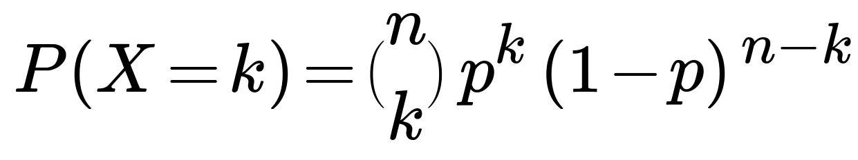
where nCk denotes the binomial coefficient “n choose k,” p is the probability of success for each trial, and (1–p) is the probability of failure.

Parameters Explanation

• n: Total number of independent Bernoulli trials.

• k: Number of successes (an integer from 0 up to n).

• p: Probability of success in each individual trial.

• 1–p: Probability of failure in each individual trial.

Computing P(X=2)

For each scenario (a, b, c, d), we calculate P(X=2) by substituting n, p, and k=2 into the formula for the binomial PMF. For instance, in (a) with n=4 and p=0.2,

P(X=2) = 4C2 × (0.2)² × (0.8)² = 6 × (0.2)² × (0.8)² = 0.1536.

Computing P(X<2)

P(X<2) means P(X=0) + P(X=1). We use the same binomial PMF for k=0 and for k=1, then sum them. For (a),

• P(X=0) = 4C0 × (0.2)⁰ × (0.8)⁴ = 1 × 1 × (0.8)⁴ = 0.4096,

• P(X=1) = 4C1 × (0.2)¹ × (0.8)³ = 4 × 0.2 × (0.8)³ = 0.4096, then add them to get 0.8192.

Computing P(X>2)

P(X>2) = 1 – P(X≤2). We already have P(X=0), P(X=1), and P(X=2). We sum them up as P(X≤2) = P(X=0) + P(X=1) + P(X=2). Then 1 minus that sum gives P(X>2). For example, in (a),

P(X>2) = 1 – [0.4096 + 0.4096 + 0.1536] = 0.0272.

We repeat these steps for the other given n and p values (b), (c), and (d).

Python Code Example

Below is a short Python snippet that illustrates how one might compute these binomial probabilities programmatically:

import math

def binomial_pmf(n, p, k):
    # Compute nCk
    nCk = math.comb(n, k)
    return nCk * (p**k) * ((1-p)**(n-k))

def compute_binomial_probabilities(n, p):
    # Probability that X=2
    p_eq_2 = binomial_pmf(n, p, 2)
    # Probability that X<2
    p_lt_2 = binomial_pmf(n, p, 0) + binomial_pmf(n, p, 1)
    # Probability that X>2
    # Another approach: p_gt_2 = 1 - (p_lt_2 + p_eq_2)
    p_gt_2 = sum(binomial_pmf(n, p, k) for k in range(3, n+1))
    return p_eq_2, p_lt_2, p_gt_2

# Example usage:
for (n, p) in [(4, 0.2), (8, 0.1), (16, 0.05), (64, 0.0125)]:
    p2, p_lt_2, p_gt_2 = compute_binomial_probabilities(n, p)
    print(f"n={n}, p={p}, P(X=2)={p2:.4f}, P(X<2)={p_lt_2:.4f}, P(X>2)={p_gt_2:.4f}")

This code confirms the numerical probabilities that we see in the short solution.

Possible Follow-up Questions

1) What is the intuition behind the binomial coefficient nCk in the binomial formula?

The binomial coefficient nCk counts the number of different ways to choose k successful trials out of n total trials. Since each subset of k successes has probability p^k * (1–p)^(n–k), you multiply that probability by the number of such subsets.

2) How would you handle the case when n is very large and p is small?

In cases where n is large and p is small, it is often computationally faster (or numerically more stable) to approximate the binomial distribution using a Poisson distribution with parameter λ = np. This is the Poisson approximation to the binomial. It works well when n is large and p is sufficiently small, so that np is moderate.

3) Could we use normal approximation instead of computing exact binomial probabilities?

Yes, the normal approximation to the binomial is also common when n is large and p is not too close to 0 or 1. One typically uses a continuity correction, so for example, P(X ≤ k) might be approximated by P(Z ≤ (k+0.5–np)/√(np*(1–p))) where Z is a standard normal variable. However, for smaller n or extreme p, the exact binomial formula or a more suitable approximation (like Poisson) is typically preferable.

4) Why do we compute P(X<2) as P(X=0)+P(X=1) but compute P(X>2) as 1 – P(X≤2)?

This is simply a matter of convenience. For X>2, one would have to sum P(X=3)+P(X=4)+…+P(X=n). Because summing every term can be tedious, it is often easier to do P(X>2) = 1 – P(X≤2). This is efficient because we already calculated P(X=0), P(X=1), and P(X=2).

5) How do we compute binomial probabilities in practice without floating-point underflow or overflow when n is large?

One strategy involves using logarithms. You can compute the log of the PMF and then exponentiate at the end. Most scientific libraries (e.g. SciPy in Python) can also do this internally and offer stable functions (like scipy.stats.binom.pmf) that handle large n without significant numerical issues.

6) How is the binomial distribution used in common machine learning scenarios?

In machine learning or statistical modeling, binomial distributions often arise in modeling the count of successes in n binary experiments—such as clicks in an online advertising setting, defect rates in manufacturing processes, or classification tasks with multiple repeated experiments. In more advanced setups, generalized linear models, like logistic regression, relate to Bernoulli trials but often incorporate predictor variables that influence p.

7) What is the relationship between Bernoulli and binomial distributions?

A Bernoulli random variable is simply a binomial random variable with n=1. In other words, a Bernoulli distribution is the special case of “one trial,” whereas binomial is “n trials.”

All these considerations reflect key knowledge for probability and basic statistical modeling that can be tested in interviews for data science or machine learning roles in major tech companies.