
ML Interview Q Series: Calculating Storage Tank Capacity Using CDF for Specific Overflow Probability
Browse all the Probability Interview Questions here.
Liquid waste produced by a factory is removed once a week. The weekly volume of waste (in thousands of gallons) is a continuous random variable with probability density function
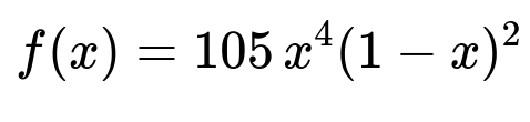
for 0 < x < 1, and f(x) = 0 otherwise. How should you choose the capacity of a storage tank so that the probability of overflow during a given week is no more than 5%?
Short Compact solution
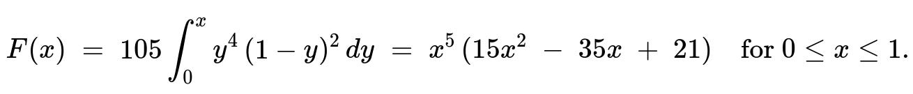
The distribution function is
We want 1 - F(x) = 0.05, which is equivalent to F(x) = 0.95. Numerically solving F(x) = 0.95 yields x = 0.8712. Hence, to keep the overflow probability at or below 5%, the storage tank capacity should be 0.8712 thousand gallons.
Comprehensive Explanation
PDF and CDF Derivation
We are given a probability density function (pdf):
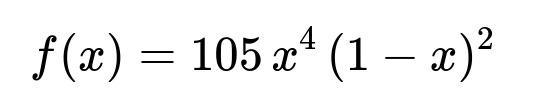
for x in (0, 1). This function resembles the form of a Beta distribution (specifically Beta(5, 3)), though we can handle it directly via integration. To find the cumulative distribution function (CDF), we integrate the pdf from 0 to x:
F(x) = integral over t from 0 to x of 105 * t^4 * (1 - t)^2 dt.
Carrying out this integration carefully (e.g., expanding t^4(1 - t)^2 to t^4 - 2 t^5 + t^6 and then integrating term by term) yields a polynomial expression in x. The resulting closed-form for the CDF is:
The domain is 0 <= x <= 1. Outside this interval, F(x) = 0 for x <= 0 and F(x) = 1 for x >= 1, given the support of the pdf.
Determining the Required Capacity
We want the probability of overflow—i.e., the probability that the weekly waste exceeds the tank’s capacity—to be at most 5%. If C is the capacity (in thousands of gallons), then mathematically this means:
Probability(X > C) = 1 - F(C) <= 0.05
or equivalently,
F(C) >= 0.95.
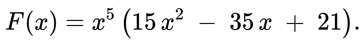
Hence we solve F(C) = 0.95. Using the closed-form expression for F(x):
C^5 (15 C^2 - 35 C + 21) = 0.95.
This polynomial equation can be tackled by any standard numerical method (e.g., Newton’s method or a simple bisection search). Numerically, the solution is approximately 0.8712. Therefore, the tank capacity must be at least 0.8712 thousand gallons (i.e., about 871.2 gallons) so that in any given week, the chance of overflow is 5% or less.
Example of Numerical Computation in Python
Below is a simple Python code snippet that numerically solves for x in F(x) = 0.95 via a bisection method:
def F(x):
    return (x**5)*(15*(x**2) - 35*x + 21)

def find_capacity(target=0.95, tol=1e-6):
    low, high = 0.0, 1.0
    while high - low > tol:
        mid = (low + high) / 2
        if F(mid) < target:
            low = mid
        else:
            high = mid
    return (low + high)/2

capacity = find_capacity()
print(capacity)
This will yield approximately 0.8712.
Follow-Up Question: Why do we trust a polynomial or Beta-type model here?
Because the pdf is only supported on (0, 1) and has a specific shape tailored to real-world measurement constraints (here, the maximum possible waste is 1 thousand gallons in a week). It is common in textbook examples or academic-style interview questions to use such a bounded polynomial distribution. In practice, you would validate whether the distribution fits actual measured data.
Answer Discussion:
Real data collection would be essential to confirm that the weekly waste is indeed bounded by 1 and behaves according to this polynomial-based pdf.
If the process changed (e.g., the factory’s production rate changed), this distribution would need re-estimation from new data.
Follow-Up Question: What if we want a different overflow probability threshold?
Sometimes 5% might be too high or too low a risk tolerance. The same method applies—if you want at most p% chance of overflow, solve:
1 - F(x) = p/100
or
F(x) = 1 - p/100
using the same polynomial expression for F(x). In more industrial settings, you might choose a smaller threshold (like 1%) or even 0.1%, depending on regulatory and operational constraints.
Follow-Up Question: Could we have solved this via Beta distribution knowledge?
Yes. Notice that f(x) = 105 x^4 (1 - x)^2 is essentially a Beta(5, 3) distribution scaled by a constant that ensures the integral over (0, 1) is 1. The Beta(a, b) distribution has pdf proportional to x^(a-1)(1 - x)^(b-1). Here, a = 5 and b = 3. The Beta(5, 3) CDF is known in closed form via the regularized incomplete Beta function. One could directly compute the quantile (95th percentile) using Beta distribution tables or statistical software. The approach would still be the same: find x such that F(x) = 0.95.
Follow-Up Question: How would you implement safety margins in a real system?
Even if the probability of exceeding 0.8712 thousand gallons is only 5%, real-world systems often introduce extra margins:
Uncertainties or changes in production might shift the distribution.
Measurement errors or possible extreme outliers might not be well-modeled by the chosen distribution.
Thus, you might choose a capacity higher than 0.8712 thousand gallons—for example, 1.0 thousand gallons—to build in extra safety. The exact margin would depend on cost-benefit analyses, risk management policies, and the severity of potential overflow consequences.
Below are additional follow-up questions
What if the actual waste volume is not bounded by 1 thousand gallons in practice?
In real manufacturing environments, it is possible that the weekly volume of waste might exceed 1 thousand gallons. This calls into question the validity of the provided pdf, which is defined only on the interval 0 < x < 1. If there is a small but non-negligible chance that the factory’s production spike or special circumstances push the waste above 1 thousand gallons, the model would underestimate the probability of overflow if we use a capacity near 1. To address this:
Data Recollection and Model Recalibration: One would need to collect empirical data to determine the maximum observed waste. If the data consistently show waste surpassing 1 thousand gallons, the bounds of the model must be extended (e.g., shifting from a Beta-type distribution to a more general distribution that can handle values greater than 1).
Tail Behavior: Even if it’s unlikely, the tail of the distribution for large x is crucial. A small chance of extremely large waste volumes can impact overflow probability significantly.
Alternative Distributions: In some cases, a lognormal or gamma distribution might capture the right-tail behavior more realistically if the true volume can sometimes spike.
Hence, simply applying the given pdf might be insufficient, and ignoring real-world unbounded extremes is a key pitfall.
Could measurement errors affect our chosen capacity?
In many industrial applications, there is inherent measurement error or instrumentation noise in the recorded waste volume. If the measurement is systematically biased or has random fluctuations, the observed distribution of weekly waste might differ from the true distribution. This discrepancy can mislead the capacity decision. To handle these concerns:
Measurement System Analysis (MSA): Determine the precision and accuracy of measurement devices. Incorporate this error into the capacity model.
Bias Correction: If a known offset or drift is discovered (e.g., always measuring 3% higher than actual), we can correct the recorded data before modeling.
Confidence Intervals: Instead of a point estimate for the 95th percentile, one might compute confidence intervals around the percentile estimate to reflect measurement and parameter uncertainties, leading to a more conservative capacity choice.
How do we address changes in the factory’s production processes over time?
The distribution of waste might shift if the factory changes production capacity, product lines, or cleaning schedules. The pdf parameters estimated from historical data might no longer apply in future weeks. This leads to potential underestimation or overestimation of the probability of overflow. To mitigate:
Non-Stationary Behavior: Model the process as potentially non-stationary; track the distribution parameters over time and update or re-estimate frequently if significant changes are detected.
Predictive Monitoring: Use control charts or anomaly detection techniques to identify distribution shifts. Once the shift is confirmed, re-derive the distribution or switch to a model that accounts for time-varying parameters (e.g., dynamic linear models or state-space models).
Contingency Plans: Maintain buffer space or flexible operational strategies (e.g., schedule additional waste pickups) if early signs of increased production are detected.
What if the Beta-like shape does not match real data at all?
Despite the neat polynomial structure, real data might reveal a different shape—perhaps the volume is more heavily concentrated at mid-range values, or it might have a multimodal characteristic if there are multiple production lines with differing waste patterns. Relying blindly on a Beta distribution form could be risky. Possible solutions:
Empirical Distribution: Use kernel density estimation or histograms to approximate the distribution directly from data. This non-parametric approach can be more flexible.
Mixture Models: If the data show multiple modes (e.g., high waste in some weeks and low waste in others), a mixture of distributions (e.g., two gamma or normal components) could better reflect this.
Goodness-of-Fit Tests: Use Kolmogorov–Smirnov or Chi-squared tests to assess how well the Beta distribution fits the empirical data before deciding on the final model.
How do we handle multiple sources of waste with different distributions?
Some factories produce waste from multiple independent production lines or processes, each with its own distribution. If you have multiple random variables X1, X2, …, representing waste volumes, you might need the sum X = X1 + X2 + … to determine total waste. Key considerations:
Convolution of Distributions: If the lines are truly independent, the total waste distribution is the convolution of the individual distributions. This might not have a simple closed form.
Simulation or Monte Carlo Methods: In many practical scenarios, one obtains the distribution of the sum by running repeated simulations. Each iteration draws a sample from each distribution and sums them, building an empirical distribution of total waste.
Dependence or Correlation: If the production lines share resources, there might be correlation. That complicates the modeling further, requiring joint distributions or copula-based approaches to accurately represent dependencies.
How would you validate that a 5% threshold is actually met in practice?
Even after solving for the capacity that theoretically holds a 5% overflow risk, real-world validation is necessary. Pitfalls include unknown distribution shifts, measurement errors, or rare extreme events not captured by historical data. A validation strategy might include:
Pilot Phase: Deploy a tank of the chosen capacity, and closely monitor actual overflow events over a trial period. If overflow events exceed the expected frequency (about 5%), investigate whether the data distribution or assumptions were incorrect.
Confidence Intervals for the Overflow Probability: Estimate the empirical overflow probability in the test period. Construct confidence intervals to see if it aligns with the 5% target.
Adaptive Refinements: If observed overflow frequency remains higher than expected, re-assess the distribution or pick a higher capacity to reduce risk further.
How might “extreme value theory” (EVT) come into play if extremely high waste values are rare but possible?
Extreme value theory deals with the statistical behavior in the tail of a distribution where rare events occur. If there is a possibility of extraordinarily large waste volume once in a long while, typical polynomial or Beta distributions might not capture the tail thickness accurately. In that scenario:
Generalized Pareto Distributions: EVT often uses these to model the tail beyond a high threshold. One might fit a high-threshold model to the largest observed weekly waste volumes and see if a heavier-tailed distribution is needed.
Block Maxima Approach: Another EVT approach is to look at maximum values over fixed time blocks (e.g., each month) to determine if the tank design is robust to these maxima.
Risk Management: Even if the probability of extremely large waste is small, the consequences (environmental damage, regulatory penalties) can be high, so tail modeling with EVT helps in capacity planning.
Could real-time monitoring and predictive analytics reduce the risk of overflow?
Instead of only installing a fixed tank size and hoping the weekly volume stays below it 95% of the time, factories might implement real-time monitoring to forecast waste generation:
Data-Driven Predictions: Use sensor data, production schedules, and machine-learning models to forecast daily or weekly waste volume. If the predicted volume is close to the tank capacity, prompt an early waste removal.
Adaptive Threshold: Update the capacity needed or the removal schedule based on dynamic production levels, thus reducing overflow risk without necessarily building an oversized tank.
Cost-Benefit Trade-Off: Real-time analytics infrastructure adds complexity and cost but can pay off by minimizing the risk of environmental incidents and potential downtime associated with overflow cleanups.
Is it possible that “5% overflow probability” itself is misleading?
When stating “the probability of overflow is 5%,” it presumes a static environment and that the distribution is well-known and stable over time. In practice, these probabilities are estimates with uncertainty:
Parameter Uncertainty: The fitted pdf might have confidence intervals around its parameters, meaning the actual cumulative distribution function could shift slightly.
Frequency vs. Probability: Observing an overflow event 2 or 3 times within 40 weeks might be within normal statistical fluctuation. Evaluating whether the actual observed rate matches the theoretical 5% can be tricky without a sufficiently large sample.
Long-Term vs. Short-Term: A 5% chance each week translates to a higher chance over multiple weeks—using that in risk calculations or multi-year predictions requires compounding the probabilities.
By clarifying these subtle points, one can ensure a more robust interpretation of the 5% target and decide if additional safety margins are worthwhile.