
ML Interview Q Series: Calculating Uniform Distribution Expectation and Variance Using Integration

Browse all the Probability Interview Questions here.
Show how to determine the expectation and the variance of a uniform distribution defined on the interval [a, b]
Short Compact solution
For a random variable X that is uniformly distributed between a and b, the probability density function is 1/(b−a). Using this density, the mean is computed by integrating x times the PDF from a to b, which gives (a + b)/2. To find the second moment, one integrates x² times the PDF over the same bounds, yielding (a² + a b + b²)/3. Substituting back into the definition of variance E[X²] − (E[X])² leads to the result (b − a)² / 12.
Comprehensive Explanation
The uniform distribution U(a, b) assumes that every point x in the interval [a, b] is equally likely. This implies that the PDF has a constant value over [a, b]. Specifically, we write:

There is zero probability mass outside [a, b], so f_X(x) = 0 elsewhere. The expectation of X is the integral of x multiplied by the PDF from a to b:
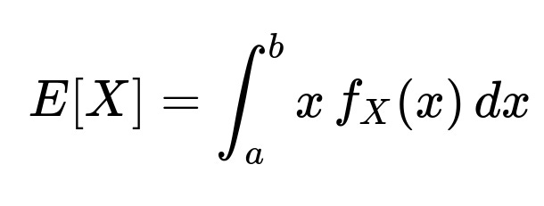
Since f_X(x) = 1/(b − a), this integral simplifies to:

One computes that integral by finding the antiderivative of x and evaluating it at the endpoints a and b. The antiderivative of x is (x²)/2, so the integral becomes ((b²)/2 − (a²)/2) / (b − a). Simplifying yields (a + b)/2. Intuitively, for a uniform distribution, the average value should lie exactly at the midpoint of the interval, and this derivation confirms that result.
To obtain the variance, one starts by calculating E[X²]:

Again, substituting f_X(x) = 1/(b − a), the integral becomes:

The antiderivative of x² is (x³)/3. Evaluating from x = a to x = b and then dividing by (b − a) leads to (a² + a b + b²)/3. Finally, variance is calculated as:

Substitute the expressions for E[X²] = (a² + a b + b²)/3 and E[X] = (a + b)/2 into the above, which simplifies to (b − a)² / 12. This is the classic result for the variance of a uniform distribution on [a, b].
This derivation holds for a < b and for all real values of a and b, whether they are positive, negative, or a mixture of both. As long as the interval is well-defined and the PDF is constant over that interval, the same formulas follow. The uniform distribution’s simplicity makes its mean the midpoint and its variance depend only on the squared width of the interval, scaled by 1/12.
Additional Follow-up Questions
What happens if the interval endpoints are negative or if a < 0 < b?
The formulas still apply. The mean will be (a + b)/2, regardless of whether a and b are positive, negative, or span zero. The variance also remains (b − a)² / 12. The location of the interval does not affect these formulas because the distribution is still uniform.
How does one handle the scenario a = b?
If a = b, the interval collapses to a single point. In that degenerate case, X takes the value a (or b) with probability 1. The mean would be a, and the variance would be zero because there is no spread. This is effectively a degenerate distribution rather than a continuous uniform distribution.
Why is the PDF 1/(b − a)?
For a uniform distribution, the total probability must be 1 over the interval [a, b]. Since it is constant in that range, one multiplies the constant by (b − a) and sets it equal to 1 to solve for that constant. This yields 1/(b − a).
How can one implement the derivations in Python?
A straightforward Python snippet illustrating the symbolic integration or direct numeric checks can be done using libraries such as sympy or numpy. One might use numpy to sample points and empirically estimate the sample mean and sample variance to confirm the analytical results:
import numpy as np

a_val = 2.0
b_val = 5.0
N = 10_000_000

# Generate uniform samples
samples = np.random.uniform(low=a_val, high=b_val, size=N)

# Compute sample mean and variance
sample_mean = np.mean(samples)
sample_variance = np.var(samples, ddof=1)  # using unbiased estimator

print("Sample Mean:", sample_mean)
print("Sample Variance:", sample_variance)

# Theoretical values:
theoretical_mean = 0.5 * (a_val + b_val)
theoretical_variance = (b_val - a_val)**2 / 12
print("Theoretical Mean:", theoretical_mean)
print("Theoretical Variance:", theoretical_variance)
One would expect the sample mean and variance to be close to the theoretical values for a large number of samples. This confirms the correctness of the mean (a + b)/2 and variance (b − a)² / 12 in a practical sense.
Are there any real-world complications in assuming data is uniformly distributed?
Real data might not follow a truly uniform distribution, so it is essential to justify whether that assumption is valid for a particular scenario. In practice, one might look at histograms, perform statistical tests, or rely on domain knowledge before concluding that data is truly uniform over an interval. Even in simulation or modeling contexts, approximating certain processes as uniform might be too simplistic. Always ensure that the uniform assumption matches domain-specific requirements and empirical evidence.
Below are additional follow-up questions
Why is the uniform distribution often chosen for bounding worst-case scenarios in practical applications?
In many engineering and risk analysis tasks, practitioners use the uniform distribution to capture minimal assumptions about variability. The logic is that if one knows only that a quantity lies between two bounds a and b but lacks any strong evidence for a more specific distribution, the uniform distribution can act as a worst-case model. Every point in [a, b] is treated as equally likely, ensuring that one does not underestimate variance or produce overly optimistic predictions. This is especially relevant for bounding errors in system design or in sensitivity analyses where we want to see the maximum possible effect that an uncertain parameter can have on an outcome.
However, a key pitfall is that a uniform distribution’s assumption of equal likelihood across the entire interval may be too simplistic. For instance, if real data cluster near a particular boundary, using a uniform model may lead to systematically inaccurate forecasts. If that clustering is significant, switching to a distribution that reflects the true empirical pattern—like a triangular or truncated normal distribution—may be more appropriate. Also, in worst-case analyses, some might prefer a distribution that places heavier weight on the boundaries (for instance, a beta distribution skewed to the edges) if boundary behaviors are truly more probable than the interior.
Could the uniform distribution be used as a prior in Bayesian inference, and what are some caveats?
Yes. In Bayesian modeling, a uniform distribution is often used as a non-informative or uninformative prior on parameters when we have no clear reason to favor one part of the parameter space over another. It encodes the idea: "All values of the parameter between the specified bounds are equally likely."
One caveat is that “non-informative” is context-dependent. A uniform prior on one scale (e.g., a parameter on the real line) might become highly informative on a transformed scale (e.g., a parameter exponentiated). This can yield misleading inferences if the parameter space is not truly best represented by that uniform assumption. Another subtlety is that, formally, a uniform prior on an unbounded domain is improper (the integral over the entire real line is infinite). Although improper priors can still yield valid posteriors, it can raise questions of whether the posterior distribution converges to a meaningful solution. Consequently, practitioners might prefer other priors (like weakly informative half-normal or half-Cauchy) that at least lightly constrain parameter values while still maintaining relative neutrality.
What about higher-order properties such as skewness and excess kurtosis for a uniform distribution?
The skewness of a distribution measures its asymmetry, and for a uniform distribution on [a, b], the skewness is zero. This happens because a uniform distribution is symmetric about its midpoint (a + b)/2, assuming a and b are finite.
The excess kurtosis of a uniform distribution is -1.2. Excess kurtosis measures how heavily the tails of a distribution differ from the normal distribution. Since the uniform distribution has finite bounds and very thin tails, its kurtosis is relatively low compared to the normal. In practical terms, this means that the uniform distribution is less "tail-heavy" than a Gaussian. Real-world data, especially in finance or social sciences, might have heavier tails than normal, so using a uniform distribution could underestimate extreme outcomes.
A subtlety is that if one tries to measure skewness or kurtosis from real data that appears to be somewhat uniform, a pure uniform model might not perfectly capture small asymmetries. Even slight deviations can lead to a non-zero skewness in practice. As with any real-world modeling, it is essential to test how well the uniform distribution really aligns with observed data before concluding that skewness is indeed zero.
If two independent U(a, b) random variables are summed, what does the resulting distribution look like?
The sum of two independent uniform random variables on [a, b] follows a symmetric triangular-like distribution, often referred to as a convolution of two uniforms. More precisely, for each possible sum y, the probability density is determined by how many ways x₁ + x₂ = y can happen with x₁, x₂ in [a, b].
If Y = X₁ + X₂, where each Xᵢ is U(a, b), then Y ranges from 2a to 2b. The PDF of Y forms a triangular shape that increases linearly from 2a up to the midpoint a + b, and then decreases linearly from a + b to 2b. This shape is sometimes called a triangular distribution. Formally, one can compute:
For y in [2a, a + b], the PDF increases from 0 to its peak.
For y in [a + b, 2b], the PDF decreases symmetrically.
A potential pitfall arises if one incorrectly assumes that the sum of two uniforms is still uniform. That assumption is false. Moreover, if the two uniform distributions differ in their intervals, one must handle the convolution carefully. Also, for sums of more than two uniform variables, the distribution evolves toward a more bell-shaped curve by the Central Limit Theorem, but the domain remains constrained by the sum of the individual intervals.
Does applying transformations to a uniform random variable help in generating other distributions, and what are the details to watch out for?
Yes. One of the most fundamental transformations is the Probability Integral Transform (PIT). If U is U(0, 1), and we set Y = F⁻¹(U), where F⁻¹ is the inverse CDF of a target distribution, then Y has that target distribution. This is a cornerstone for simulation and is commonly employed with techniques like the inverse transform sampling method in Monte Carlo simulations.
Potential pitfalls involve discontinuities or undefined sections of the inverse CDF. If F is not strictly increasing or has plateaus, the inverse transform method might need more careful handling. Also, if one has only a uniform distribution on [a, b] instead of [0, 1], then scaling to [0, 1] is usually performed as (X − a)/(b − a) before applying the inverse CDF. Additionally, numerical inaccuracies can arise for extreme values if the function or its inverse is not well-behaved or if floating-point precision is limited.