
ML Interview Q Series: Calculating Lognormal Expected Value Using Moment Generating Functions.

Browse all the Probability Interview Questions here.
Consider a random variable X such that log(X) is normally distributed with mean 0 and variance 1. Find the expected value of X.
Short Compact solution
Let Y = log(X). Our goal is to compute E[X], which is E[e^Y]. Since Y ~ N(0, 1), the moment generating function (MGF) of Y at s is given by exp(s² / 2). Evaluating this MGF at s = 1 gives exp(1/2). Hence E[X] = exp(1/2).
Comprehensive Explanation
Lognormal Distribution Overview
When a random variable X is said to have a log(X) that follows a Normal distribution (in other words, if log(X) ~ N(μ, σ²)), then X is called a lognormal random variable. The property that log(X) is normally distributed has major implications for X’s statistical behavior, including its moments.
Here, we have the special case where μ = 0 and σ² = 1, which means log(X) ~ N(0, 1). This is often referred to informally as "X ~ Lognormal(0,1)."
Expectation Computation Using MGF
One direct method to find E[X] is to observe that X = e^Y, so:
Y = log(X)
E[X] = E[e^Y]
For a Normal random variable Y ~ N(0, 1), its MGF is given by
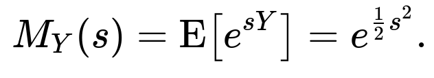
This is a known result for any Normal(0,1) variable. If we want E[e^Y], we need M_Y(1). Thus:

Hence, for this lognormal variable, the mean is simply exp(1/2).
Interpretation and Intuition
Since log(X) ~ N(0, 1), the "center" of log(X) is 0. This would suggest that on a logarithmic scale, X is equally likely to be above or below 1 when measured in log-scale.
However, exponential transformations are not linear, so the distribution of X is skewed to the right. Hence the actual average E[X] is greater than 1 and equals e^(1/2).
Practical Considerations
In real-world scenarios, lognormal distributions commonly model positive-valued data that spans several orders of magnitude, such as time-to-failure in reliability studies, financial asset prices under certain assumptions, or certain types of measured data in biology and engineering.
If we wanted to validate this theory empirically, we could run a Monte Carlo simulation where we draw samples Y from N(0,1), then take X = exp(Y), and compute the sample mean of X to see if it approximates e^(1/2).
import numpy as np

N = 10_000_000
Y_samples = np.random.normal(loc=0.0, scale=1.0, size=N)
X_samples = np.exp(Y_samples)
print(np.mean(X_samples))  # Should be close to np.exp(0.5)
What If Y ~ N(μ, σ²)?
If we generalize to the case log(X) ~ N(μ, σ²), then by the same reasoning, E[X] = exp(μ + σ²/2). In our specific question, μ = 0 and σ² = 1, so E[X] = exp(1/2).
Potential Edge Cases
X must be strictly positive if log(X) is well-defined in the usual sense. Hence, any real-world data leading to negative or zero values cannot be modeled directly by a lognormal distribution.
Numerical underflow or overflow can occur if X is extremely large or small in practical computations.
Common Interview Follow-Up Questions
How do we interpret “log(X) ~ N(0,1)” in terms of X itself?
If log(X) follows a normal distribution with mean 0 and variance 1, it means that the variable X is lognormal. For each outcome x, log(x) lies on a bell-curve shape centered at 0. In practical terms, X is positive and can become very large, although most values cluster around e^0 = 1.
Can we derive the moment generating function of Y more explicitly?
For Y ~ N(0,1):
The probability density function (pdf) is

A well-known result from Gaussian integrals is that this integral evaluates to exp(s² / 2). If the interviewer asks for the step-by-step derivation, you would typically complete the square in the exponent and use standard integral identities for the normal distribution.
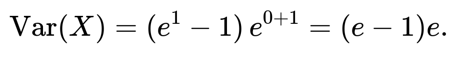
What is the variance of X when X = e^Y and Y ~ N(0,1)?
The variance of a lognormal variable X when Y ~ N(μ, σ²) is

For our case (μ = 0, σ² = 1), it simplifies to e( e - 1 ). Precisely:

Why is the mean not simply exp(0) = 1, since the mean of log(X) is 0?
Because the relationship between X and log(X) is exponential (which is nonlinear), the expectation of X is not the exponential of the expectation of log(X). Instead, there is an additional variance-related term in the exponent that causes E[X] to exceed exp(0).
How could one approximate E[X] from sample data in practice?
To approximate E[X] using observed samples x₁, x₂, …, xₙ from the distribution, you would compute the sample average:
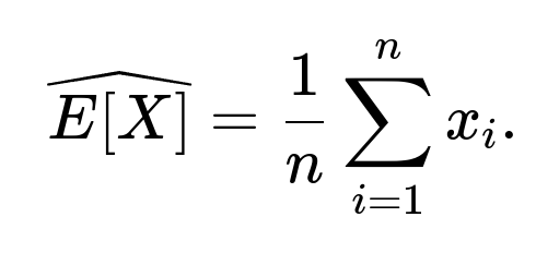
However, if your data is heavily skewed, you might also consider using robust statistics or taking logs of the data to see if it appears normally distributed in log-space. This log-transformation is often used to reduce skewness and simplify variance modeling.
Could we have used the fact that X is lognormal directly?
Yes. A well-known formula for a lognormal random variable X with parameters μ and σ² is E[X] = exp(μ + σ²/2). Knowing this identity is often sufficient for an immediate answer. However, in many interviews, showing the MGF approach (or at least referencing it) demonstrates stronger mathematical understanding.
Are there any numerical or computational pitfalls?
For extremely large or small values of Y, exp(Y) might overflow or underflow in floating-point arithmetic. To mitigate this, data scientists sometimes employ techniques such as working in log-space until the final calculation step, or using libraries that handle extended precision. In typical double-precision scenarios, floating-point overflow occurs when the exponent is beyond around 709 (for exp(709) ~ 8.2184e307 in Python).
How might this question appear in a machine learning context?
In certain regression tasks (log-linear models), we may assume the log of the target variable is normal. Then the predictions effectively target log(y), but after training, predictions are exponentiated to return to the original scale. Understanding that E[e^(Predicted_log(Y))] ≠ e^(mean(Predicted_log(Y))) clarifies why “log-space predictions” can systematically bias your final predictions and how to adjust them if you want an unbiased estimate of the mean on the original scale.
All these considerations often arise in advanced modeling and data analysis scenarios where lognormal assumptions are made about the data-generating process.
Below are additional follow-up questions
What if our data includes non-positive values, even though we assumed X is lognormal?
When assuming log(X) ~ N(0, 1), we require X > 0 because the logarithm is undefined for non-positive values. In practical datasets, however, zeros or negative values can arise due to measurement errors, domain mismatches, or data-collection peculiarities. These scenarios create serious challenges:
Data Preprocessing: One possible workaround is to shift the data by a positive constant before applying the log transform (e.g., use log(X + c) for some c > 0), but this distorts the interpretation slightly since the distribution is no longer a simple lognormal.
Measurement Error Modeling: Sometimes zero or negative readings might indicate noise or truncated measurement instrumentation. In that case, you might incorporate a “censoring” or “truncation” model, rather than treating these data points as out-of-distribution anomalies.
Model Invalidity: If a substantial portion of the data is ≤ 0, the lognormal assumption may not be appropriate at all. An alternative positive-valued model (like Gamma or a zero-inflated approach, if many zeros exist) might be more realistic.
Edge Case Detection: In an interview, you might be asked to propose how to handle negative or zero data. Showing an understanding that a raw log transform is invalid in such cases demonstrates familiarity with real-world data issues.
How can we verify empirically if log(X) is actually normally distributed?
In practice, we rarely know for certain that log(X) has a perfect normal distribution. To assess this:
Histogram or Density Plot:
Transform your observed data to Yᵢ = log(Xᵢ) for each sample Xᵢ > 0.
Plot a histogram or kernel density estimate of {Yᵢ}. If it roughly looks bell-shaped, that’s a qualitative indicator.
Q-Q Plot (Quantile-Quantile Plot):
Compare the empirical quantiles of Y = log(X) to the theoretical quantiles of a N(0,1) distribution (or to a N(μ, σ²) if you have an estimated mean μ and standard deviation σ of Y).
If the points closely follow the 45° line, log(X) is probably close to normally distributed.
Statistical Tests:
Use formal tests (e.g., Shapiro-Wilk, Kolmogorov-Smirnov, Anderson-Darling) on Y = log(X). A failure to reject normality does not guarantee perfect normality, but it adds confidence.
Box-Cox or Other Power Transforms:
If log transformation doesn’t yield an approximate normal distribution, alternative transforms (Box-Cox, Yeo-Johnson, etc.) might do better.
Practical Significance:
Even if log(X) is not perfectly normal, slight deviations might be tolerable. Overly strict demands on normality might be less critical if the model predictions are still robust in practice.
Could outliers in X distort the assumption that log(X) ~ Normal?
Yes, extreme outliers in X can seriously affect the distribution of log(X), though taking logs often reduces the impact of large outliers by compressing the scale. Still:
Impact of Extreme High Values:
If X contains extremely large values, the log transform may reduce their scale but might still leave the tail heavier than a standard normal tail.
In certain domains (e.g., finance), sudden spikes can create “fat-tailed” distributions even after logs.
Presence of Spurious Outliers:
Sometimes outliers are measurement artifacts or data-entry errors. Carefully investigate these points; if they are erroneous, removing or correcting them is preferable to blindly forcing the lognormal model.
Robust Estimation:
One might use robust estimators (e.g., robust mean estimators, robust standard deviation estimators) or heavier-tailed distributions if outliers are genuine but frequent.
How do correlations with other variables behave if X is assumed lognormal?
Correlation analysis often becomes subtler when variables are lognormal:
Linear Correlation vs. Log-space Correlation:
If X is lognormal, a linear correlation with another random variable Y might not be meaningful if Y is measured on a linear scale. Instead, we might consider correlation in log-space, i.e., corr(log(X), Y).
In many scenarios (e.g., analyzing returns in finance or analyzing size scales in biology), it’s more interpretable to examine correlation between log-transformed variables.
Nonlinear Associations:
Because log transforms are nonlinear, the relationship between X and another variable might look curved in raw scale but become more linear in log scale.
Modeling Covariates:
When you build regression or machine learning models that assume log(X) is normal, you also implicitly assume that the linear relationships hold in log-space. If the candidate is asked about how to incorporate multiple predictors, you might mention generalized linear models or transformations of both the predictors and the response to maintain linearity.
Does the lognormal distribution apply if X has an upper bound?
Lognormal distributions are unbounded above; theoretically, they stretch to infinity. If your real-world variable X has a strict upper limit (e.g., a saturation threshold for a physical measurement), pure lognormal modeling may not fully capture that constraint:
Truncated Lognormal:
Sometimes, you can treat the variable as lognormal truncated at an upper bound. This requires specialized truncated-likelihood calculations.
Alternative Distributions:
In a domain where boundedness is strict (for instance, percentages between 0 and 1, or concentrations that can’t exceed solubility limits), a Beta distribution or a bounded transformation might be more appropriate.
Practical Workaround:
If the bound is so high that only an extremely small fraction of data approach it, the lognormal model might still be an acceptable approximation in practice. Always check how often your data nears the boundary.
Is it possible for the lognormal assumption to hold only in a particular range of X values?
Yes, real-world data can exhibit “piecewise” distributions, where a lognormal assumption might hold only within certain segments:
Multimodal Situations:
If the data are generated from multiple processes, each might follow a lognormal distribution with different parameters. In that case, a single lognormal fit across the entire data range won’t capture the multimodality.
Threshold or Regime Effects:
In some fields (like hydrology or precipitation modeling), X can be near zero often (rainfall is zero on many days), then heavy on some days, with a lognormal tail beyond some threshold. A single lognormal for all X can be incorrect. Mixture distributions (e.g., a point mass at zero plus a lognormal for X > 0) might be needed.
Diagnostics:
Plotting log(X) or using a Q-Q plot restricted to different intervals can reveal if only one part of the data is consistent with normality in log-space.
In advanced modeling, you might define piecewise transformations or separate distributions for different intervals.
How to choose between lognormal and other distributions (e.g., Gamma, Weibull) when modeling positive data?
Even though lognormal is a common choice, it’s not always the best:
Domain Knowledge:
Certain phenomena have theoretical justifications for specific distributions. For instance, waiting times for Poisson processes are often better modeled by an exponential or Gamma distribution. Material strength might be well-modeled by Weibull.
Lognormal might come from multiplicative processes where the exponent of repeated multiplication becomes normally distributed.
Model Fit Criteria:
Compare candidate distributions through goodness-of-fit tests (e.g., likelihood-based metrics like AIC/BIC, or KS/Anderson-Darling tests).
If multiple distributions seem plausible, evaluating them with out-of-sample predictions or cross-validation can help decide.
Tail Behavior:
Lognormal can have heavier or lighter tails compared to Gamma or Weibull, depending on parameter settings. Real data that exhibit “long tails” might be better aligned with a lognormal or certain heavy-tailed distributions.
Robustness & Interpretability:
Log transformations are widely familiar and often used in statistical and machine learning contexts. Gamma or Weibull might be more specialized.
Decision-makers in certain industries prefer or are used to specific models, factoring into practical distribution choice.
How do Bayesian methods handle lognormal assumptions for X?
In a Bayesian setup, you might place a prior on log(X) rather than X itself:
Prior on Mean and Variance in Log-space:
You can place a normal prior on μ and an inverse-gamma or half-Cauchy prior on σ². The posterior then incorporates observed data Xᵢ > 0. The likelihood term uses the lognormal pdf.
Sampling:
Markov Chain Monte Carlo (MCMC) or Variational Inference methods will typically sample log(X) or the underlying normal parameters directly. This can be convenient, as sampling in log-space might lead to fewer sampling issues, especially if X can span multiple orders of magnitude.
Inference for Derived Quantities:
If you need E[X], or Xᵢ predictions, you can transform posterior samples from log(X) back to the original scale. However, be mindful that the posterior distribution for X is typically skewed.
Pitfalls:
Bayesian inference can still struggle if the data has zeros, negative measurements, or significant truncation. You would either exclude those points or design an appropriate data-generating model that accounts for them.
Could an extreme multiplicative process invalidate the standard lognormal assumption?
A lognormal model often arises from the Central Limit Theorem for multiplicative processes: if X is the product of many independent, positive factors, then log(X) is the sum of their logs, often leading to approximate normality in log-space.
Heavy-Tailed Multiplicative Processes:
If the factors have heavy-tailed distributions themselves or are not independent, the sum of logs might not converge to a normal distribution. This can create distributions heavier-tailed than the conventional lognormal.
Mix of Additive + Multiplicative:
Real phenomena might be partly additive and partly multiplicative. For instance, X might be = (Baseline + Noise) × (Multiplicative Factor). In that case, log(X) might not be strictly normal.
Empirical Check:
Again, the best approach is to check the empirical distribution of log(X). If it deviates systematically from normal, consider other transformations or more flexible distributions (e.g., log-t distribution for heavier tails).
How does one simulate multiple correlated lognormal variables?
If an interviewer extends the question to higher dimensions:
Joint Distribution:
Suppose you have random variables X₁ = e^Y₁ and X₂ = e^Y₂ where (Y₁, Y₂) jointly follow a bivariate normal distribution with a certain correlation ρ. Then (X₁, X₂) are said to have a “multivariate lognormal” distribution.
Practical Implementation:
Generate correlated normal pairs (Y₁, Y₂) by constructing a covariance matrix:

Then exponentiate each dimension to get (X₁, X₂).
Challenges:
Real data might show correlation in a nonlinear way. Merely matching correlation of log(X) might not fully capture complex dependencies.
If you require more than pairwise correlation or more intricate dependence structure, you might resort to copulas or more elaborate joint modeling approaches.


What if the sample size is very small—can we still rely on the lognormal assumption?
Small sample sizes complicate any distributional assumption, including lognormal:
Parameter Estimation Variance:
Estimating μ and σ² from just a few log-transformed samples can produce large uncertainty. In small-sample scenarios, outliers have a more pronounced effect.
Bootstrapping:
With limited data, resampling techniques might help approximate the variability of estimates. However, bootstrap methods also rely on having enough representative data.
Robustness and Prior Information:
In a Bayesian framework, imposing an informative prior for μ and σ² might stabilize estimates when data is scarce. Alternatively, domain knowledge that strongly suggests lognormal behavior can lend confidence in the assumption, even if n is small.
Practical Recommendation:
If the interviewer probes further, you might discuss using approximate methods or acknowledging that with limited data, the distribution fit is uncertain. Additional data collection might be more beneficial than overfitting an assumption to a tiny dataset.