ML Interview Q Series: Calculating the Correlation Coefficient Between Counts of Different Die Faces

Browse all the Probability Interview Questions here.

28. Say you roll a fair die 5 times. Let X be the count of times a 2 appears, and Y be the count of times a 3 appears. What is the correlation coefficient between X and Y?

Detailed Explanation of the Solution

Understanding the problem We roll a fair six-sided die 5 times, and each roll is an independent event. X is the total number of times we get the face 2, and Y is the total number of times we get the face 3. Both X and Y are random variables that depend on the same set of 5 rolls. Intuitively, X and Y should be negatively correlated: if you roll more 2’s, that leaves fewer opportunities to roll 3’s (and vice versa).

Defining X and Y more formally We can write each random variable as a sum of indicator variables across the 5 rolls:

Let the outcomes be denoted as roll 1, roll 2, ..., roll 5. Define an indicator for roll i:

• Iᵢ = 1 if roll i = 2, and 0 otherwise.

• Jᵢ = 1 if roll i = 3, and 0 otherwise.

Then,

X = I₁ + I₂ + I₃ + I₄ + I₅ Y = J₁ + J₂ + J₃ + J₄ + J₅

Each Iᵢ is a Bernoulli(1/6) random variable (with probability 1/6 of being 1 for a given roll), and similarly each Jᵢ is Bernoulli(1/6). However, note that Iᵢ and Jᵢ for the same i cannot both be 1 simultaneously (because a single roll can’t be 2 and 3 at the same time).

Expected values The expectation of X is the sum of the expectations of each Iᵢ:

E[X] = E[I₁ + I₂ + I₃ + I₄ + I₅] = 5 × (1/6) = 5/6

Similarly,

E[Y] = 5/6

Variance of X and Y Because each roll is independent from the others, for X we have:

Var(X) = Var(I₁ + I₂ + ... + I₅) = 5 × (1/6) × (5/6) = 25/36

Likewise,

Var(Y) = 25/36

Covariance of X and Y We use the definition:

First, consider X·Y:

X·Y = (I₁ + ... + I₅) × (J₁ + ... + J₅)

This expands to:

I₁J₁ + I₁J₂ + ... + I₅J₄ + I₅J₅

We split it into two kinds of terms:

1. Terms where i = j, which look like Iᵢ Jᵢ. Because a single roll cannot be both 2 and 3, Iᵢ and Jᵢ cannot both be 1. Hence for any single roll,

Iᵢ Jᵢ = 0

So each term Iᵢ Jᵢ has expectation 0.

2. Terms where i ≠ j. For i ≠ j, Iᵢ and Jⱼ refer to different rolls (which are independent events). The probability that roll i is 2 (Iᵢ=1) is 1/6, and the probability that roll j is 3 (Jⱼ=1) is 1/6, so

E[Iᵢ Jⱼ] = P(Iᵢ=1) × P(Jⱼ=1) = (1/6) × (1/6) = 1/36

There are 5 × 5 = 25 total pairs (i, j). Among these, 5 pairs have i = j, leaving 20 pairs with i ≠ j. Hence,

E[XY] = E[ ∑(i ≠ j) Iᵢ Jⱼ ] = 20 × (1/36) = 20/36 = 5/9

Therefore,

and

E[X] E[Y] = (5/6) × (5/6) = 25/36, 5/9 = 20/36,

So,

Cov(X, Y) = 20/36 - 25/36 = -5/36

Correlation coefficient The correlation coefficient between X and Y is:

Since Var(X) = 25/36 and Var(Y) = 25/36, we get

√Var(X) = 5/6 and √Var(Y) = 5/6, so √(Var(X) Var(Y)) = (5/6)(5/6) = 25/36.

Thus,

Hence, the correlation coefficient is -1/5.

Interpretation of the result The negative correlation of -1/5 tells us that if you get more 2’s than “usual,” there’s a slight tendency to get fewer 3’s, but the effect is moderate (not extremely close to -1). Conceptually, every time you roll a 2, that roll could otherwise have been a 3, so X and Y compete for outcomes across the 5 trials.

Could you verify the correlation with a simulation in Python?

Certainly. Below is an illustrative simulation to empirically estimate the correlation. We will simulate a large number of 5-roll sequences, count the number of 2’s (X) and 3’s (Y), and then compute the sample correlation coefficient.

import random
import statistics

def simulate_correlation(num_simulations=10_000_00):
    # We'll store values of X and Y from each simulation
    x_values = []
    y_values = []

    for _ in range(num_simulations):
        rolls = [random.randint(1, 6) for _ in range(5)]
        x = sum(1 for r in rolls if r == 2)
        y = sum(1 for r in rolls if r == 3)
        x_values.append(x)
        y_values.append(y)

    return statistics.correlation(x_values, y_values)

estimated_corr = simulate_correlation()
print("Estimated correlation:", estimated_corr)

If you run this code (with a suitably large number of simulations), you should see the correlation converge close to -0.2, which supports our theoretical derivation of -1/5.

Are X and Y independent random variables?

They are not independent. Intuitively, if you roll more 2’s in those 5 trials, it leaves fewer opportunities to roll 3’s. The covariance formula (and negative sign) captures that effect. If they were independent, we would expect E[XY] = E[X] E[Y] exactly, implying Cov(X, Y) = 0, but that is not the case here (we got -5/36).

Why is the correlation negative?

Because the events “roll a 2” and “roll a 3” for the same trial are mutually exclusive, increasing the count of 2’s (X) implies you have fewer rolls left to produce 3’s (Y), and vice versa. This competition for the same trials leads to a negative association. Rolling a 2 on a particular trial precludes rolling a 3 in that same trial.

Why exactly -1/5?

The -1/5 arises from the specific arithmetic that involves:

• Each X and Y has expected value 5/6.

• Each variance is 25/36.

• The Cov(X, Y) ended up being -5/36.

Once you divide -5/36 by 25/36, the 36 cancels out, leaving -5/25 = -1/5. This fraction is determined by two factors: (1) the fact that the probability for each face is 1/6, and (2) the number of trials is 5. If either changed, the correlation would be different.

Could the correlation be -1?

No. -1 would mean a perfect negative linear relationship, which can’t happen for these counts. Even if you get extra 2’s, you can still get some 3’s as well, just with somewhat lower expectation. The maximum possible negative correlation for two discrete count variables in a small-sample scenario is not going to be -1; there are only 5 trials in total, and that leaves room for random variation in outcomes. Hence, we end up with a moderate negative correlation of -1/5.

How does this generalize to more dice rolls or more faces?

If we roll n times, let Xᵢ be the count of a certain face i. For face i and face j, the correlation would follow the same reasoning: each count has a Binomial(n, 1/6) distribution if the die is fair. The expected covariance depends on whether the events can occur simultaneously on a single trial (they cannot if we are counting two distinct faces). The negative correlation would scale in a way related to n and p=1/6. In general, if you have multiple outcomes in each trial that cannot overlap, the correlation between counts of distinct outcomes is negative, and you could compute it in the exact same manner:

E[XY] would involve the probability that different rolls produce the respective faces, minus the product of expectations.

What if we assumed independence incorrectly?

If you assume X and Y were independent, you might reason incorrectly that Cov(X, Y) = 0. This leads to a flawed assumption about the distribution. For instance, in certain statistical tests or modeling approaches, if you treat these counts as though they do not interact, you would underestimate the negative relationship that arises from these two events being mutually exclusive per single trial.

Misapplying a model that assumes X and Y are independent can cause errors in analyzing how the counts move together. It’s a subtle detail: each trial picks exactly one face, so events are not independent in terms of how they distribute among possible faces.

Could you use X to predict Y?

In principle, you could set up a simple linear regression of Y on X, since they are negatively correlated. However, the relationship is modest (correlation -0.2). On average, you might find that if X is unexpectedly high, Y might be slightly lower than expected, but the predictive power would not be very strong. This is because many other faces (1, 4, 5, 6) also occur, and the random variation across just 5 rolls is quite large.

You can still interpret the regression line to see that for each unit increase in X (i.e., one extra 2), you would expect a small decrement in Y on average. But again, 5 trials is a small sample, and the correlation is not extremely large in magnitude.

Summary of key points

X (number of 2’s) and Y (number of 3’s) over 5 fair die rolls have:

• E[X] = 5/6, E[Y] = 5/6

• Var(X) = 25/36, Var(Y) = 25/36

• Cov(X, Y) = -5/36

• Correlation coefficient = -1/5

Hence, the correlation coefficient is exactly -0.2.

Below are additional follow-up questions

If the die were not fair, how would we compute the correlation coefficient between X and Y?

To handle a scenario with a biased die, let the probability of rolling a 2 be denoted by p, and the probability of rolling a 3 be denoted by q. Since a single die roll can yield one of six faces, we must also account for the probabilities of rolling any of the other faces. The main difference from the fair-die case (p = q = 1/6) is that these probabilities may no longer be 1/6.

Defining the random variables in the biased case X is still the total count of 2’s in 5 rolls. Y is still the total count of 3’s in those 5 rolls. We can again express them as sums of indicator variables:

Let Iᵢ = 1 if roll i = 2, 0 otherwise, with probability p of being 1. Let Jᵢ = 1 if roll i = 3, 0 otherwise, with probability q of being 1.

Then X = I₁ + I₂ + I₃ + I₄ + I₅ and Y = J₁ + J₂ + J₃ + J₄ + J₅.

Expected values E[X] = 5p E[Y] = 5q

Variances Each X is the sum of independent Bernoulli(p) variables, hence Var(X) = 5 p (1 - p) Similarly, Var(Y) = 5 q (1 - q)

Covariance One must consider that Iᵢ and Jᵢ for the same roll i cannot both be 1, because a single outcome can’t be “2” and “3” simultaneously. So:

1. For i = j, E[IᵢJᵢ] = 0 because the events “roll = 2” and “roll = 3” for the same roll can’t co-occur.

2. For i ≠ j, Iᵢ and Jⱼ are independent Bernoulli variables with probabilities p and q, respectively. Thus E[Iᵢ Jⱼ] = p × q for i ≠ j.

There are 5 × 5 = 25 total pairs (i, j). Among them, 5 have i = j and 20 have i ≠ j. Therefore:

E[XY] = E[∑(i ≠ j) Iᵢ Jⱼ] = 20 × p × q

Hence,

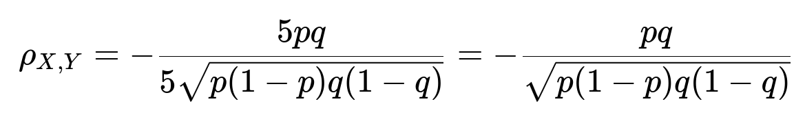
Cov(X, Y) = E[XY] - E[X]E[Y] = 20 p q - (5p)(5q) = 20 p q - 25 p q = -5 p q

Finally, the correlation coefficient becomes:

In simplified form:

Interpreting the result Because p and q are probabilities for mutually exclusive outcomes on a single trial, the sign of the covariance remains negative. If p and q are quite large (and still less than 1), the magnitude might be different from the fair-die case, but the relationship is still negative so long as 2 and 3 can’t appear on the same roll.

Pitfalls and edge cases One edge case is if p + q > 1. That’s impossible for a single six-sided die if p is the probability of rolling 2 and q is the probability of rolling 3, but if we contrive some other scenario, we must ensure that the sum of all face probabilities = 1. Another subtle pitfall is if p or q approaches 0 or 1. That can make the correlation formula approach boundary behaviors. For example, if p = 0, then X is almost always 0, leading to zero variance and an undefined correlation.

Real-world analogy A biased die might reflect a scenario where certain outcomes are more likely. The negative correlation generalizes seamlessly from the fair-die scenario, but the exact value depends on p and q in the manner shown above.

How do we derive a joint probability mass function for X and Y, and can that help validate the correlation?

We can consider the complete joint distribution P(X = x, Y = y) for x, y = 0, 1, 2, 3, 4, 5, subject to x + y ≤ 5 because you can’t have more than 5 rolls in total. For each outcome, x means you specifically got 2 on x rolls, y means you specifically got 3 on y rolls, and the remaining (5 - x - y) rolls must be something else.

General structure of the joint pmf If the die is fair, the probability of rolling a 2 is 1/6, rolling a 3 is 1/6, and rolling anything else is 4/6. Then the probability that exactly x of them are 2, y of them are 3, and the remaining 5 - x - y are neither 2 nor 3 is given by:

for x + y ≤ 5. Zero otherwise.

Validating correlation through the joint pmf Once you have the joint pmf, you can compute E[X], E[Y], E[XY], etc., directly from summations over x and y. Summing x × y × P(X = x, Y = y) yields E[XY]. Similarly, summing x × P(X = x, Y = y) over x and y yields E[X], and so on. Checking that the result matches the known -1/5 correlation (in the fair case) is a good validation.

Potential pitfalls One subtlety is ensuring x + y ≤ 5. Another is that each (x, y) pair must be accounted for in the multinomial coefficient. If a person tries to treat X and Y as though they could independently range up to 5, they might incorrectly include pairs like (x = 5, y = 5), which is impossible. Another subtlety is to remember that rolling a 2 on a particular trial excludes rolling a 3 on that same trial.

Real-world perspective In a multi-class classification setting, the joint pmf is akin to a distribution of how often each class label appears. This distribution-based approach can help you compute correlations between pairs of classes if you consider “count of predicted class i” and “count of predicted class j” across multiple trials.

How does the correlation change if we consider more than two faces, for instance, X is the count of 2’s, Y is the count of 3’s, and Z is the count of 4’s?

When we introduce Z as the count of 4’s, we have three random variables that measure how many times we get 2, 3, or 4 in 5 rolls of a fair die. Each pair among (X, Y, Z) will exhibit a negative covariance, for the same reason: any given trial that contributes to X = 1 for that trial cannot simultaneously contribute to Y = 1 or Z = 1, and so on. Generally, for a fair die:

E[X] = E[Y] = E[Z] = 5/6 Var(X) = Var(Y) = Var(Z) = 5 × (1/6) × (5/6) = 25/36 Cov(X, Y), Cov(X, Z), Cov(Y, Z) all become negative. Each pair can be computed by the same logic that got us -5/36.

Potential pitfalls Confusion can arise if one tries to sum up pairwise correlations incorrectly or assume they sum to a certain number. Also, with three or more variables, you can talk about partial correlations, which measure the correlation of two variables after controlling for the effect of a third. That can shift the sign or magnitude. Another pitfall is mixing up covariance with correlation: Cov(X, Z) might be the same in magnitude as Cov(X, Y), but correlation depends on each pair’s standard deviations.

Real-world analogy In multi-class problems (like multi-label classification or multi-outcome experiments), you can have multiple “counts” that measure how many times each label or category was selected. You often find that these counts are negatively correlated because each trial can produce only one category. This general idea extends to anything from dice rolls to user selection of one brand out of several choices.

If we transform X and Y (for instance, consider X² or log(X+1)), how does that affect the correlation?

Correlation specifically refers to a linear relationship measure between the original random variables X and Y. If you transform them, the correlation typically changes or might even become undefined if you transform values that can be zero or negative in ways that break continuity. Examples:

Squared transformation If you consider X² and Y², they do not move linearly with X and Y. Hence the correlation between X² and Y² is generally different from Corr(X, Y). The sign can even change or become near zero.

Log transformation If you define U = log(X+1) and V = log(Y+1), the correlation between U and V can be quite different from Corr(X, Y). The reason is that the log function compresses large values more than small values, which can alter linear relationships.

Pitfalls One pitfall is to assume that a monotonic transformation of X or Y preserves correlation. Spearman’s rank correlation might remain positive/negative if the transformation is monotonic, but Pearson’s correlation measure is about the covariance of X and Y in a linear sense, so transformations can drastically change it. Another pitfall is applying a transform that is not well-defined for X=0 or for negative values (though negative X is not possible here, we might have X=0, so log(X) is not well-defined unless we shift by +1).

Real-world perspective When counts have a heavy-tailed distribution, transformations like log can be helpful for modeling. But always be sure to check if the linear relationship is still captured or if you need a different correlation measure (like Spearman correlation).

If we only observe partial rolls (say we lose track of some rolls) but still want to estimate correlation, what happens?

Consider a scenario where 5 rolls occur, but we only observe 3 of them. The other 2 are unobserved or missing. We want to estimate the correlation between the count of 2’s and the count of 3’s from incomplete data.

Estimating with missing data A naive approach might be to ignore the missing data, but that typically biases the correlation estimate. Another approach is to use an expectation-maximization (EM) method, or multiple imputation, to fill in plausible values for the missing outcomes. In each imputed or EM iteration, you guess the distribution of unobserved outcomes and compute an updated estimate of correlation.

Pitfalls If the data are not missing at random, the correlation might be severely biased. For example, if you selectively missed recording a roll only when it was a 2, your data systematically undercounts 2’s and might skew the correlation. Another subtlety is that the typical formula for correlation assumes you have complete pairs of measurements. With missing data, you no longer have full knowledge of the pair (X, Y). You need a more robust statistical method.

Real-world analogy In large-scale data problems, missing data can be quite common. If we treat missing outcomes incorrectly, we might incorrectly conclude that there is no correlation or a weaker correlation. Knowing how to handle that properly is a hallmark of good data analysis in classification tasks, A/B testing, or even online experimentation with partial logs.

What if we define a new variable W = 5 - (X + Y)? How does that interact with X and Y?

W could be interpreted as the count of rolls that are neither 2 nor 3. Then we have:

X + Y + W = 5

All three random variables are determined from the same set of 5 rolls. The presence of W ensures that for any triple (x, y, w), they must sum to 5. Each pair (X, W), (Y, W), (X, Y) will exhibit negative correlation. Also, X, Y, and W are not mutually independent because you can’t choose x, y, and w freely—they must satisfy x + y + w = 5.

Why define W? Sometimes you’re interested in not just how many times you get 2 or 3, but also how many times you get something else. This W can reveal if the negative correlation might become clearer when you consider the tri-variate distribution. For example, rolling many 2’s or 3’s leaves fewer remaining rolls for W to capture.

Pitfalls It’s easy to double-count or forget constraints in enumerating possible outcomes. Another pitfall is that W can be correlated with X or Y in a negative way, because if X is high, W is likely lower. That can complicate multi-variate analyses if you assume independence.

Real-world context In multi-class classification with 3 classes, each trial belongs exactly to one class. The variables (X, Y, W) measure how many times each class label was assigned. It’s typical that these variables can’t be independent, and correlation or negative dependence arises from the same “one trial, one outcome” logic.

If we repeated the 5-roll experiment multiple times (each set of 5 rolls is one “block”) and computed the correlation for each block, how would we assess stability or confidence intervals?

In practice, you might not rely on the theoretical result alone but gather empirical data from repeated sets of 5 rolls. Suppose you do M blocks of 5-roll sequences, record (Xᵢ, Yᵢ) for i = 1, ..., M, and then compute the sample correlation across these M blocks:

1. Each block i yields an (Xᵢ, Yᵢ).

2. We compute the sample correlation from the M data points.

Confidence intervals You can then use standard statistical techniques to form a confidence interval around that sample correlation. For instance, the Fisher z-transformation method: transform sample correlations to a z-scale, compute standard errors, and transform back.

Potential pitfalls If M is not large, the sample correlation can deviate notably from the true -1/5. Another subtlety is the distribution of (X, Y): it’s multinomial in each block. If M is large, we expect the sample correlation to converge near -1/5, but for small M, you might see strong sampling variability.

Real-world perspective When analyzing correlation from repeated discrete experiments, it’s important to gather enough repeated “blocks” so that the sample correlation is stable. Over a small number of blocks, spurious correlations might appear.

How does the concept of correlation here compare with mutual information between X and Y?

Correlation (specifically Pearson’s correlation) is a measure of linear dependence. Mutual information is a more general measure of how much knowledge of one variable reduces uncertainty about the other. Even if correlation is zero, mutual information can still be positive if there’s a nonlinear or more complicated relationship.

In this scenario (5 rolls, X = count of 2’s, Y = count of 3’s): They do have negative correlation. But they also have strictly positive mutual information because knowing how many times we rolled a 2 definitely reduces the uncertainty of how many times we rolled a 3 (they cannot overlap in a single trial).

Potential pitfalls Sometimes, seeing a correlation of zero in other contexts might mislead someone to think there’s “no relationship.” But mutual information can capture all forms of dependence, including those that aren’t linear. Here, the correlation is negative, so both correlation and mutual information show dependency. But if you had a different scenario with no linear relationship but still some constraints that reduce uncertainty, correlation might be zero while mutual information is nonzero.

Real-world analogy In classification tasks, mutual information between two class counts can still be positive even if the correlation is minimal, because there might be constraints or more complex relationships that do not show up in a linear correlation measure.

Is it possible for the correlation between X and Y to be zero if we define X and Y differently, but still counting events over 5 rolls?

Yes, it can happen if X and Y are defined in such a way that the constraints do not force a negative or positive dependence. For instance, consider:

X = number of times we roll an even face (2, 4, 6) Y = number of times we roll a prime face (2, 3, 5)

In that scenario, you can get overlap for face = 2, because that belongs to both sets (it’s even and prime). A single roll that is 2 increments both X and Y. There’s a partial synergy in those events, and also a partial exclusivity if you roll a 4 or 6 for X but not Y, or a 3 or 5 for Y but not X. The sign of that correlation is not trivially guaranteed to be negative. In some contrived definitions of X and Y, one can achieve zero or near-zero correlation.

Pitfalls It’s easy to assume that any two counts from the same set of trials must be negatively correlated, but that’s not necessarily true if events can overlap or partially overlap (like a single roll can increment both counts). Another subtlety is whether the same trial can contribute to both X and Y. That is usually the deciding factor in whether the correlation is forced negative, forced positive, or is ambiguous.

Real-world analogy Consider a multi-label classification problem where certain labels can co-occur for the same item. Then the counts of each label might exhibit positive correlation if they often appear together in the same item. So, the sign of correlation depends heavily on whether the label sets overlap.

How does this discrete correlation example relate to the concept of a hypergeometric distribution, and is there any scenario where we might use that?

A hypergeometric distribution typically arises when we sample without replacement from a finite population. In a sense, each die roll is sampling from the set of possible outcomes, but it’s with replacement. The correlation we see here is partly reminiscent of negative dependence that arises in hypergeometric setups: when you draw a “success,” it reduces the number of successes left in a finite population. However, for dice rolling, each trial is independent in terms of physical mechanics.

Nonetheless, if you had a scenario akin to drawing from an urn with 2’s and 3’s, the negative dependence might be even stronger because you physically remove each success from the population. Then X and Y might have an even more pronounced negative correlation.

Potential pitfalls Don’t conflate the dice scenario (independent trials) with a hypergeometric scenario (sampling without replacement). The negative correlation in the dice example arises from the logical impossibility of rolling two distinct faces on the same trial. With hypergeometric sampling, the negative correlation arises from physically depleting a finite resource of “successes.” They are conceptually linked by the notion that events can’t co-occur in one draw, but the underlying distributions and formulas differ.

Real-world viewpoint Understanding both binomial/multinomial models (for with-replacement or repeated independent trials) and hypergeometric models (for without-replacement sampling) is vital in experimental design. If you misapply one distribution to a scenario that fits the other, you can incorrectly compute correlation or probability statements.

Could the correlation be reversed in sign if we allow each roll to have multiple simultaneous outcomes in a more general scenario?

Yes. If in some hypothetical scenario each roll can yield multiple “labels” simultaneously (which is not physically true for a standard six-sided die, but might be true in multi-label classification tasks where each item can belong to multiple classes), then the correlation sign could flip. For example, if we define:

X = number of times label A appears in a set of items Y = number of times label B appears in the same set of items

and items can have both label A and label B simultaneously, that co-occurrence can induce a positive correlation. The correlation sign depends on whether events can or cannot occur together.

Pitfalls In dice-based logic, it’s easy to assume different outcomes are mutually exclusive for the same trial. But in a generalized scenario where outcomes or labels can co-occur, you must carefully check whether the correlation is necessarily negative or not. Another pitfall is applying the formula for negative covariance from the dice scenario to a multi-label scenario where events can overlap. This can lead to erroneous conclusions.

Real-world example In a recommendation system, a user might watch multiple categories of videos simultaneously or might watch content that falls under both “comedy” and “romance.” The counts of how many times a user consumed each genre are often positively correlated. By contrast, in the single-outcome dice scenario, the correlation is negative because outcomes can’t overlap within the same trial.

Could we consider a Bayesian approach to estimate the correlation of X and Y, and would that differ from the frequentist approach?

Yes. In a Bayesian framework, you would specify priors over the probabilities of rolling 2 (p) and rolling 3 (q). You would then observe the counts of 2’s and 3’s in a series of 5-roll experiments, update your posterior distributions over (p, q), and use the posterior distribution to derive a posterior distribution for the correlation.

Mechanics of a Bayesian approach

1. Start with a Dirichlet prior for the six faces of the die, or a Beta prior for p if you only focus on the probability of rolling a 2, similarly for q.

2. Observe the actual data: how many times each face is rolled.

3. Update the posterior distribution over (p, q).

4. Then for each sample (p*, q*) from the posterior, compute the correlation implied by those p*, q*.

5. Summarize the distribution of correlation, e.g., with posterior mean or credible interval.

Pitfalls You must be careful about the prior you choose. If you pick an extremely biased prior or an improper prior, your posterior correlation might be skewed. Another subtlety is that in a single 5-roll experiment, you might not get enough data to precisely pin down p and q. The correlation might remain uncertain.

Real-world perspective A Bayesian viewpoint can be especially helpful if you suspect the die might be biased or if you want to combine prior knowledge (for instance, from historical data about dice or from a calibration test). You can also incorporate hierarchical models if you suspect partial biases in multiple dice or contexts.

How would the correlation coefficient behave if we considered a very large number of rolls (n → ∞)? Does it vanish?

Let’s generalize to n rolls and define X as the count of times we roll a 2, Y as the count of times we roll a 3. For a fair die,

E[X] = n/6 E[Y] = n/6 Var(X) = n × (1/6)(5/6) = 5n/36 Var(Y) = 5n/36 Cov(X, Y) = ?

We can apply the same logic as before: out of n² total (i, j) pairs, n are i = j. For i ≠ j, the events are independent. The fraction of i = j pairs is negligible as n grows large, but you still have exactly n pairs that yield zero contribution (for i = j, the probability roll i is 2 and roll j is 3 is impossible). So:

E[XY] ~ (n² - n)(1/6)(1/6) plus the i=j terms that are zero. That’s roughly n²/36 minus some lower-order terms. Meanwhile, E[X]E[Y] = (n/6)(n/6) = n² / 36. The difference (E[XY] - E[X]E[Y]) ends up approximately -n/36. More precisely, it’s -5n/36 when you carry out the exact count for the i≠j pairs.

Thus Cov(X, Y) ~ -5n/36, and the correlation is:

Wait, that might seem contradictory to the earlier formula, so let’s be precise: The exact formula for Cov(X, Y) when we have n trials is:

Cov(X, Y) = E[XY] - E[X]E[Y]. We find E[XY] = (number of i≠j pairs) × P(roll i=2, roll j=3) = (n)(n-1)(1/6)(1/6) + 0 for the i=j terms. That’s (n)(n-1)/36. So E[XY] = n(n-1)/36. Meanwhile, E[X]E[Y] = (n/6)(n/6) = n²/36.

Hence Cov(X, Y) = [n(n-1)/36] - [n²/36] = [n² - n - n²]/36 = -n/36. Then Var(X) = n(1/6)(5/6) = 5n/36, similarly Var(Y) = 5n/36.

So the correlation is:

It remains -1/5, even as n → ∞. That matches the logic from the 5-roll scenario, except now it’s n rolls. So it does not vanish and does not approach -1; it remains a constant negative correlation of -1/5 for a fair die, for any finite n.

Pitfalls A naive guess might be that “as n grows, maybe X and Y converge to their means, so the correlation might vanish.” But that’s not the case. The negative correlation is a structural feature: each trial forbids rolling 2 and 3 simultaneously, so the fraction of times we get a 2 is inversely related to the fraction of times we get a 3. Another pitfall is incorrectly handling the combinatorics or mixing up the n(n-1) terms.

Real-world perspective In repeated multi-outcome trials, some forms of competition remain no matter how large n is. The correlation can stay nonzero because the underlying exclusivity is always present at each trial.

How can we misinterpret the meaning of negative correlation if we only have small data for X and Y?

When you collect only a small number of sets of 5-roll experiments, you might see wide fluctuations in sample correlation. Even though the “true” correlation is -1/5, your empirical correlation from a handful of blocks could be positive by chance or might be extremely negative.

Potential misinterpretation Someone might see an empirical correlation of -0.5 from a small data set and conclude the relationship is quite negative. Another might see +0.1 from an even smaller or different sample and think they’re uncorrelated or even slightly positively correlated. This highlights how correlation estimates can be noisy with small sample sizes.

Edge cases If, in a small sample of rolls, you happen to roll a lot of 2’s but also a lot of 3’s (though improbable, it can happen with randomness), the sample correlation might appear less negative or even positive. If you consistently fail to roll any 2’s or 3’s in that small sample, the correlation might be undefined or close to 0 if X and Y are often zero simultaneously.

Real-world analogy In any data science scenario with small sample size, sample correlations can be misleading or unstable. Confidence intervals become very wide. One might incorrectly dismiss or overstate an underlying dependence. Checking theoretical reasoning or running large enough experiments is vital to avoid misinterpretation.

How does knowledge of correlation between two faces scale up if we want the full correlation matrix among all six faces?

Define X₁ as the count of face 1, X₂ as the count of face 2, and so on, up to X₆ as the count of face 6, each over n rolls. We can build a 6×6 covariance matrix Σ describing Cov(Xᵢ, Xⱼ). For a fair die:

E[Xᵢ] = n/6 Var(Xᵢ] = n(1/6)(5/6) = 5n/36 If i ≠ j, Cov(Xᵢ, Xⱼ) = ?

Since each trial can produce exactly one face, the negative correlation extends to any pair of distinct faces. By the same combinatorial argument, Cov(Xᵢ, Xⱼ) = -n/36 for i ≠ j. Therefore, the correlation matrix will have 1 on the diagonal (once we standardize each variable by its standard deviation √[5n/36]) and the same negative off-diagonal entries that correspond to -1/5.

Practical meaning This means that in a fair-die scenario with many possible outcomes, all different faces are equally negatively correlated, because each face is equally likely and each face is mutually exclusive with every other face.

Pitfalls In real data that might appear to have “faces,” you could see a structure that’s not equi-probable or equi-correlated. If the process generating the data is not truly symmetrical, the correlation matrix can become more complicated. Another subtlety is ensuring you’re consistent about the fact that each trial yields exactly one outcome, so the row sums (in a “one-hot encoding” sense) are always 1 for each trial.

Real-world analogy In multi-class classification with 6 classes, the confusion matrix of predicted classes might reflect the negative correlations in how many times each class is chosen overall. If you measure Xᵢ = “how many times model predicted class i,” these Xᵢ’s typically sum to n. Pairs of classes are negatively correlated in the sense described above, but the magnitude depends on how frequently the model chooses each class.

How do boundary cases like n=1 or n=2 highlight the limitations of correlation?

For n=1: X and Y can each only be 0 or 1. The possible outcomes for that single roll are 1, 2, 3, 4, 5, or 6. If X=1, that means the roll was 2, so Y must be 0. If Y=1, that means the roll was 3, so X must be 0. If the roll is anything else, X=0 and Y=0 simultaneously. The correlation concept in that single trial is somewhat degenerate. You can still compute a correlation, but it will often be an odd or not particularly meaningful value because X and Y might both be 0 (in which case the correlation is not well-defined if you only have one sample overall).

For n=2: We have a bit more room but still a small set of possible outcomes. The correlation is still theoretically negative, but the sample correlation from one experiment of 2 rolls is extremely variable. If you only do a single 2-roll experiment, you might get X=1 and Y=1 (which is impossible in a single roll, but across two rolls it can happen if the first roll is 2 and the second roll is 3). That might suggest no clear negative correlation in that small sample. Over repeated 2-roll blocks, though, the average correlation would approach the theoretical value if you aggregated enough such blocks.

Pitfalls Interpreting correlation from extremely small n is tricky because you can have limited or zero variance in the data. Another subtlety is that with n=1, it’s not clear how to define correlation after the fact, because you might just have a single data point or extremely limited variation. So, conceptually, correlation is best interpreted in contexts where you have more trials or repeated “blocks” of trials.

Real-world analogy In some quick pilot tests with only a few samples, your correlation measures can be meaningless. Large enough sampling is necessary for correlation to be a stable estimate of linear dependence. You might need either a single large block (n large) or multiple moderate-sized blocks to average out the noise.