ML Interview Q Series: Calculating PMF for Highest Woman's Rank Using Combinatorics

Browse all the Probability Interview Questions here.

Five men and five women are ranked according to their scores on an exam. Assume that no two scores are the same and all possible rankings are equally likely. Let the random variable X be the highest ranking achieved by a woman. What is the probability mass function of X?

Short Compact solution

Using a counting argument over all 10! equally likely rankings, the probability that the highest-ranking woman occupies the first position is found by counting 5×9! permutations over the total 10! permutations, giving 5/10. Similarly, for the highest-ranking woman to occupy the second position, one man is placed in the first position (5 choices), then a woman in second, and permutations of the remaining 8 people, yielding 5×4×8!/10! = 5/18. Continuing this pattern yields:

Alternatively, by thinking of drawing 5 blue balls (women) and 5 red balls (men) one by one without replacement, X can be interpreted as the draw on which the first blue ball appears. Because it cannot appear later than the 6th draw (all 5 red balls would have already appeared in the first 5 draws if no blue ball appeared earlier), the same distribution emerges via conditional probability arguments.

Comprehensive Explanation

Understanding the Problem

We have 10 distinct individuals: 5 men and 5 women. They are ranked in order of their exam scores (with rank 1 being the best). We define a random variable X to be the “highest ranking achieved by a woman,” which, due to the convention of rank 1 being the best, translates to “the smallest rank index that a woman attains.”

Because there are 5 men and 5 women, the highest ranking for a woman must be at least 1 (if a woman takes the top spot) and at most 6 (if all top 5 are men and the best woman is in position 6).

Counting Approach

All 10 individuals can be permuted in 10! ways, and each permutation is equally likely. To compute the probability that X = i, we need to count how many permutations have the best-ranked woman in position i, with all better ranks occupied by men.

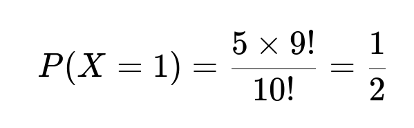
For X=1, we choose any of the 5 women for the top position. The remaining 9 slots can be occupied by the other 9 individuals in any order. Hence the count of favorable permutations is 5×9!. Dividing by the total 10! permutations gives:

For X=2, we must place a man in rank 1 (5 choices), then place one of the 5 women in rank 2, and permute the remaining 8 individuals arbitrarily (8! ways). Thus, 5×4×8! total permutations. Dividing by 10!:

Continuing similarly, the number of men occupying ranks before i changes as i increases, giving the remaining terms of the probability mass function. This approach matches the short solution above.

“Balls in a Bag” (Conditional Probability) Approach

An alternative viewpoint is that we place 5 red balls (representing men) and 5 blue balls (representing women) in a bag. We draw balls one at a time without replacement and note the position of the first blue ball. That position is effectively the highest ranking achieved by a woman.

To see why X cannot exceed 6, consider that if you do not see a blue ball in the first 5 draws, then you have drawn all 5 red balls already, so the earliest time to see a blue ball is the 6th draw.

Concretely, P(X=1) is the probability that the first draw is a blue ball: 5/10. Then,

P(X=2) is the probability that the first ball is red (5/10) and the second ball is blue (5/9). So:

5/10 * 5/9 = 5/18.

One can proceed similarly for positions 3, 4, 5, and 6, always multiplying the probabilities of drawing red balls first, then drawing a blue ball. This yields the same answers as the counting approach.

Why the Distribution Must Sum to 1

A quick sanity check is to add P(X=1) through P(X=6):

1/2 + 5/18 + 5/36 + 5/84 + 5/252 + 1/252 = 1

This confirms the probabilities cover all scenarios (woman is best in rank 1, or 2, or 3, or 4, or 5, or 6) and no other rank is possible for the best woman.

Intuition Behind the Result

The “highest ranking achieved by a woman” is a random variable that depends on how interspersed men and women are in the final sorted ranking. Because the number of men and women is equal, it is relatively likely that a woman ranks in the top few positions (note that P(X=1) = 1/2 is quite large). As we move further down the list, the probability becomes smaller because it requires that multiple men occupy the very top positions consecutively.

Potential Follow-Up Questions

How does the formula change if there are m men and w women, with m > w?

When we generalize to an unequal number of men and women, the highest rank a woman can achieve is at most w+1 if m >= w. For instance, if there were 6 men and 5 women, the highest possible rank for a woman is position 6 if all top 5 are men. The same counting logic applies, but the probabilities shift to account for the new ways of distributing men among top positions. One would count permutations in which exactly k men occupy the top k ranks, followed by a woman, or use a conditional probability viewpoint with a bag of 6 red and 5 blue balls.

What if ties are possible?

In typical exam rankings, ties force a different interpretation of “rank.” Here, the scenario was simplified by assuming no two people share the same score. In the presence of ties, the notion of a single “highest rank for a woman” becomes more complicated: multiple women could tie for first place, so we would need a suitable definition of the random variable (e.g., is it the numeric rank assigned to all tied top scorers?). The combinatorial count or bag-pull analogy would require a careful adjustment to handle identical outcomes.

Could we verify this distribution via simulation?

Yes, it is straightforward to do a Monte Carlo simulation in Python. We can randomly permute 10 distinct labels (say M1, M2, M3, M4, M5, W1, W2, W3, W4, W5) many times, record the best-ranked woman, and empirically compute the frequency of X=1, X=2, …, X=6. That frequency should approximate the exact probabilities.

import math
import random
from collections import Counter

N = 10_000_000
counts = Counter()

people = ['M1','M2','M3','M4','M5','W1','W2','W3','W4','W5']

for _ in range(N):
    perm = random.sample(people, 10)
    # Find the rank of the first woman
    for i, person in enumerate(perm):
        if person.startswith('W'):
            counts[i+1] += 1
            break

for i in range(1, 7):
    print(f'X = {i}, Empirical P: {counts[i]/N}')

Running such code for a sufficiently large number of trials confirms the theoretical probabilities (5/10, 5/18, 5/36, 5/84, 5/252, 1/252) within a small margin of simulation error.

Below are additional follow-up questions

What is the expected value of X?

To find E(X), note that X can take values 1 through 6. We can use the probability mass function P(X = i) that we already derived:

1. X = 1 with probability 5/10

2. X = 2 with probability 5/18

3. X = 3 with probability 5/36

4. X = 4 with probability 5/84

5. X = 5 with probability 5/252

6. X = 6 with probability 1/252

The expected value is the sum over all possible i of i * P(X = i). In a more general setting for 5 men and 5 women, we could also adopt the “balls in a bag” approach to derive E(X) without enumerating every term explicitly:

We can write: E(X) = 1P(X=1) + 2P(X=2) + ... + 6*P(X=6).

Once those numerical values are computed, they will sum to the exact expectation. A potential pitfall is when the total number of men or women changes, the maximum possible X also changes, so the summation boundaries must be updated accordingly.

In many real-world scenarios, the expectation of “best rank for a certain subgroup” can help an organization set realistic benchmarks or diversity goals in contexts like test scores or hiring. One subtlety is ensuring ranks are truly comparable across individuals with different backgrounds or different test conditions (e.g., different versions of exams). Another potential issue is that ties or approximate ties can complicate the distribution, and the closed-form approach might need modification.

If X were defined as the highest ranking achieved by a man, how would that change the result?

If we let Y be the highest ranking achieved by a man, then the distribution effectively flips because we have 5 men and 5 women. By symmetry, the distribution of Y is identical to X’s distribution when men and women swap roles. In this particular problem, there are 5 men and 5 women, so P(Y = 1) is also 1/2, and the rest follow similarly. The potential pitfall is to mistakenly assume that X and Y are somehow complementary in the sense X + Y = 11 or something similar. That’s not correct, because they are separate random variables describing two different events.

In real-life interview or exam contexts, “highest ranking man” might coincide with “highest ranking woman” if we define them differently (especially when ties occur). Another subtlety is that if there were more men than women, or vice versa, the symmetrical distribution no longer holds.

Can we frame this using a hypergeometric distribution directly?

Yes. One might view the position of the first woman (i.e., X) through the lens of hypergeometric probabilities. In a hypergeometric setting, consider the event “the first i−1 positions are all men” and “the ith position is a woman.” The probability of all men in the first i−1 positions is:

(number of ways to choose i−1 men from 5 men) × (number of ways to choose 0 women from 5 women) divided by (number of ways to choose i−1 individuals from all 10 people)

Then, for the ith position to be a woman, we would look at how many women remain, how many total people remain, and so on. One possible pitfall is to forget that once you fix the first i−1 positions as men, the ith position is a single woman, and the rest can be any arrangement of the remaining 9−(i−1) people. The combinatorial reasoning can be slightly trickier than the straightforward 10! ratio method, so it’s a subtlety that needs careful attention. This perspective, however, can be helpful to see how the hypergeometric distribution matches the same result as the “balls in a bag” approach.

What is the probability that at least one woman is in the top 3 positions?

Sometimes, an interviewer might ask for a probability that a certain number of women appear in the top k ranks. For “at least one woman in the top 3,” we can use complementary counting: compute the probability that all top 3 positions are occupied by men and subtract from 1. There are 5 men and 5 women total, so:

• Probability that top 3 are all men = (number of ways to choose 3 men out of 5 men) × (number of ways to choose remaining 7 out of the total 7 people left) / (number of ways to choose any 10 out of 10).

But in simpler terms, because no two scores are the same, it becomes a direct permutation problem:

Number of ways to choose and order 3 men from 5 men × number of ways to order the remaining 7 people divided by the number of ways to order all 10 people.

A subtlety arises if we had more men than women (e.g., 6 men, 4 women), we would have to adjust the counting carefully. Another pitfall is forgetting that “top 3 are men” includes multiple permutations of those men, not just combinations. This question highlights how the base problem can be extended to more general queries of the distribution of men and women among top ranks.

Does the distribution of X still hold if the exam is curved or scaled differently for different subgroups?

In real life, some exams might be curved (scaled differently) across subgroups. If men and women’s scores are not identically distributed or not equally likely, then the assumption of “all orderings equally likely” no longer holds. The result that P(X=1) = 1/2, etc., relies on the principle that all 10! permutations are equally likely. If men on average scored differently from women, then the rankings would be biased toward one subgroup. A big subtlety is that if the underlying distribution of men’s and women’s scores is not uniform, the combinatorial approach (or the “balls in a bag” approach with equal probabilities) is no longer valid. Instead, we would need to integrate over the distribution of scores or apply alternative models (e.g., normal distributions with different means).

How can we quickly verify the result for smaller numbers?

A frequent reality check is to try an even simpler case, such as 2 men and 2 women. In that scenario, the highest-ranked woman X can be 1, 2, or 3 at most (because if the top 2 ranks are men, the best woman would be in rank 3). We can enumerate all permutations easily:

• M1, M2, W1, W2

• M1, W1, M2, W2

• M1, W1, W2, M2

• W1, M1, M2, W2 ... etc.

By systematically counting in a small case, we verify the logic for the entire distribution. Pitfalls here include forgetting some permutations or incorrectly labeling them. This ensures that for the bigger 5 men/5 women scenario, the pattern of reasoning stands.

What if we are interested in the distribution of the second-best woman’s rank?

Let us define Y as the rank of the second-best woman. We now have to consider that the best woman could be in some rank i, and then the second-best woman could be in a rank j > i. Enumerating all 10! permutations directly is possible but more involved. Alternatively, we can use conditional probability, conditioning on the event X = i for the best woman. Once the best woman is placed, we look at how the remaining 4 women and 5 men are distributed among ranks i+1 through 10. The second-best woman is then the best among those 4 women in that subset of positions.

The subtlety here is that to handle Y properly, we must track the distribution of men and women among the remaining 9 positions. This can be extended to the third-best woman, etc. In real-world interviews, this question might test a candidate’s ability to manage multi-step conditioning without confusion.

How might real testing or ranking scenarios break the assumption of all permutations being equally likely?

In many practical testing scenarios:

• Participants might have varying expected performances based on prior knowledge or socio-economic factors.

• The test might not be purely random; certain systematic biases could skew the distribution.

• There might be partial credit, retakes, or other testing conditions that violate the “no ties” assumption.

Hence, the neat combinatorial solution assumes a perfect uniform distribution over all possible rankings. In reality, exam results often follow a distribution that does not guarantee the same probability for each ordering, which means the classic formula for P(X = i) is no longer exactly correct. One subtlety is that if there are latent correlations (e.g., men from certain backgrounds scoring similarly, or the top scorers are disproportionately from a certain subgroup), the independence and uniform-likelihood assumption is invalid. This can be addressed by building a probabilistic model for performance, though that becomes far more complex than the straightforward combinatorial approach.

What if, after the exam, we only know partial rank information (e.g., we only know which five individuals are in the top 5, but not the order within those top 5)?

This is a more nuanced data-availability scenario. If we only know that the top 5 are a certain set of people (men and/or women) but do not know their exact relative ordering, we can’t directly determine the “highest ranking woman.” We might only know whether at least one woman is in the top 5. From an interview perspective, the question might shift to: “Given partial knowledge of the rank distribution, what is our posterior probability distribution for X?” We can apply conditional probability or Bayesian updating to reflect the newly available partial information (e.g., “We know the top 5 contain 3 men and 2 women. What’s P(X=1) under that partial info?”).

A potential pitfall is to assume that knowing the identity of some top scorers is the same as fully specifying which rank each person got. In real-world ranking systems, partial information (like only knowing who made the ‘shortlist’ but not their exact rank) is common. We must carefully define which conditional events we are using and how that changes the total space of equally likely permutations.