ML Interview Q Series: Calculating Unfair Coin Probability with Bayesian Inference After Five Tails.

Browse all the Probability Interview Questions here.

13. There is a fair coin (one side heads, one side tails) and an unfair coin (both sides tails). You pick one at random, flip it 5 times, and observe that it comes up tails all five times. What is the chance that you are flipping the unfair coin?

This problem was asked by Facebook.

To solve this, we typically use a Bayesian inference approach. We have two hypotheses:

• Hypothesis U: You picked the unfair coin (the double-tailed coin). • Hypothesis F: You picked the fair coin (one side heads, one side tails).

You start with a prior probability of picking either coin:

Then you observe 5 tails in a row. Let T_5 denote the event of "5 tails in a row."

Under Hypothesis U (the unfair coin), the probability of flipping tails 5 times in a row is 1, because the unfair coin will always land tails:

Under Hypothesis F (the fair coin), the probability of flipping tails 5 times in a row is

We apply Bayes’ theorem:

Substituting the values:

• (P(T_5 \mid \text{U}) = 1) • (P(T_5 \mid \text{F}) = 1/32) • (P(\text{U}) = 0.5) • (P(\text{F}) = 0.5)

We get:

Numerically, this simplifies to

So the probability that the coin you are flipping is the unfair coin, given that you observed 5 tails in a row, is ( \frac{32}{33} \approx 0.9697).

An intuitive interpretation is that it is very unlikely (though not impossible) for a fair coin to produce 5 tails in a row, whereas for the double-tailed coin it happens with certainty. Observing these tails strongly suggests (with probability 32/33) that you chose the unfair coin.

Below is a short Python code snippet to illustrate this calculation:

import math

# Prior probabilities
p_unfair = 0.5
p_fair = 0.5

# Likelihoods
p_5tails_unfair = 1.0       # Probability of 5 tails with unfair coin
p_5tails_fair   = (1/2)**5  # Probability of 5 tails with fair coin

# Apply Bayes' rule
posterior_unfair = (p_unfair * p_5tails_unfair) / (p_unfair * p_5tails_unfair + p_fair * p_5tails_fair)
print(posterior_unfair)  # Should print 0.9696969696... i.e. 32/33

Below are possible follow-up questions a FANG-level interviewer might ask about this problem and comprehensive, in-depth answers to each.

How would the answer change if we observed a different number of tails, say 4 tails out of 5 flips?

If you observe 4 tails out of 5 flips, the Bayesian formula still applies, but the likelihood terms change. You would have:

• Probability of 4 tails out of 5 flips with the unfair coin (U): Because the unfair coin cannot produce heads at all, the probability of exactly 4 tails and 1 head is actually 0. If the coin truly has both sides tails, you would never see a head.

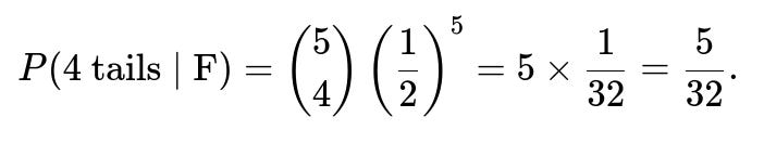
• Probability of 4 tails out of 5 flips with the fair coin (F): This is given by the binomial probability

In this scenario:

• (P(T_4, H_1 \mid \text{U}) = 0). • (P(T_4, H_1 \mid \text{F}) = 5/32).

Hence, if you truly observed exactly 4 tails and 1 head, the posterior probability of having chosen the unfair coin becomes 0. Because the event you observed could not have happened with the double-tailed coin, Bayesian updating would produce:

The intuition is straightforward: if you see any heads at all, you can immediately rule out the double-tailed coin.

What if the coin was not perfectly fair but had probability p of landing heads? How would the formula generalize?

When the coin is not perfectly fair, we have:

• Probability that the coin is the "two-tailed" coin: still 0.5 prior. • Probability that the coin is the "biased coin" with probability (p) of heads: 0.5 prior.

If we observe 5 tails in a row, the likelihood under the biased coin is

The likelihood under the double-tailed coin is still 1. Substituting into Bayes’ theorem:

You can simplify:

As (p) gets smaller (which means the coin is more likely to produce tails), ((1 - p)^5) gets larger, and (P(\text{unfair coin} \mid T_5)) goes down accordingly. Conversely, if (p=0.5) (the fair case), this formula becomes the (\frac{32}{33}) example you originally computed. If (p) is large (a coin biased heavily towards heads), then ((1 - p)^5) is small, making it more likely that seeing many tails indicates the two-tailed coin.

Why is this a Bayesian inference problem, and could we solve it without explicitly invoking Bayes’ theorem?

This problem is fundamentally Bayesian because you have:

• A prior distribution over which coin you have (equal chance of fair vs. unfair). • An observed outcome (5 tails). • A need to compute a posterior probability (the probability of having the unfair coin given the observed data).

Any approach that tries to find the probability of “unfair coin given 5 tails” is effectively a Bayesian approach. Sometimes people solve it by reasoning about the ratio of probabilities of seeing the evidence (likelihood ratio) and then normalizing over all possibilities, which is in essence exactly Bayes’ theorem in disguise. Hence, any correct solution that calculates “chance of having the unfair coin after seeing the data” is necessarily Bayesian, even if you don’t label it as such.

An alternative perspective—though mathematically the same—would be to say: • Out of all the times you could randomly pick the fair or unfair coin and then see 5 tails in a row, what fraction of those times come from the unfair coin? That perspective leads to the same calculation but is simply a more direct counting argument (think of flipping a coin to decide which coin you have, then flipping that coin 5 times, and seeing in which fraction of outcomes you get TTTTT from the unfair coin vs. from the fair coin).

Could there be real-world complications in interpreting these probabilities?

Yes, several potential real-world complications or pitfalls might arise:

• The prior probabilities might not be exactly 0.5 and 0.5. For instance, maybe you had background information about how often each type of coin is in a jar, or you suspect that someone is more likely to give you a normal coin than a trick coin. That would change (P(\text{U})) and (P(\text{F})).

• You might not trust your observation fully—perhaps you didn’t see the coin flips carefully, or the coin could have been dropped in a corner, etc. If you have some uncertainty about the outcome (like maybe one flip was suspiciously dropped under a table), that complicates your likelihood model.

• Each coin flip is assumed independent. In practice, physical coin flips can sometimes have subtle biases or dependencies if they’re not flipped fairly or if the coin is manipulated.

In a strict interview puzzle sense, we ignore these complications and treat the scenario as an idealized Bayesian problem with independence, perfect knowledge of the coin structure, and correct observation of 5 tails.

If instead of 5 flips, we flipped the coin n times and observed n tails, how would we express the posterior probability in general form?

Let (T_n) be the event of observing (n) tails in (n) flips. With the same prior probabilities of 0.5 and 0.5 for the unfair and fair coin:

• (P(T_n \mid \text{unfair}) = 1). • (P(T_n \mid \text{fair}) = \left(\frac{1}{2}\right)^n).

By Bayes’ theorem:

$$P(\text{unfair} \mid T_n)

= \frac{1 \times 0.5}{1 \times 0.5 + \left(\frac{1}{2}\right)^n \times 0.5} = \frac{0.5}{0.5 + 0.5 \times (1/2)^n} = \frac{1}{1 + (1/2)^n}.$$

So in the general case,

As (n) grows large, ((1/2)^n) gets very small, and the posterior probability of the unfair coin grows closer and closer to 1. In other words, the more tails you see in a row, the more evidence you gather that the coin is likely to be the double-tailed one.

What if in practice the “unfair” coin had some tiny chance of landing heads, and we only approximated it as having no heads?

Sometimes you see real-world trick coins where they are heavily biased towards tails but not absolutely guaranteed. In that scenario, your prior model might treat the “unfair” coin as (P(\text{heads})=\epsilon) for some small (\epsilon). That would change your likelihood calculation for the unfair coin to something close to but not exactly 1 for repeated tails. Specifically:

By updating with the correct likelihood, you’d get a posterior that is still high but not 1 if you see multiple tails. The principle remains: the more precise your model, the more accurate your Bayesian inference. However, in many classic puzzle or interview settings, the coin is either truly fair or truly double-tailed with no heads possible, so we treat it as probability 1 for tails in the unfair case.

Could we mistakenly reason that seeing 5 tails with a fair coin is impossible and jump to 100% conclusion?

Yes, that is a common error in some naive approaches. Indeed, it is not impossible for a fair coin to produce 5 tails; the probability is ((1/2)^5 = 1/32). While 1/32 is small, it is still nonzero. One must therefore weight it relative to the unconditional probability from the double-tailed coin. Bayes’ theorem ensures you never prematurely assign 100% to any hypothesis unless that event is literally impossible under every other hypothesis.

In this problem, we see that even with 5 tails in a row, there remains a small chance ((1/33)\approx 3%) that you did get unlucky with a fair coin. This is exactly what the 32/33 posterior for the unfair coin means: about a 3% chance it’s the fair coin that just happened to show 5 tails in a row.

How can I ensure no mistakes in a real interview when explaining?

In a FANG-level interview, clarity and correctness are crucial. Some best practices:

• State your assumptions (prior probabilities, independence, etc.). • Write out the Bayesian formula and carefully place the terms. • Substitute numeric values slowly and double-check arithmetic. • Provide a short intuitive reasoning (“the chance of 5 tails with a fair coin is small, so it heavily favors the double-tailed coin”).

Showing that you understand each step and can reason about possible pitfalls (like forgetting to apply Bayes’ theorem or incorrectly computing binomial probabilities) proves your depth of knowledge in data science and statistical reasoning.

Summary of the final answer

Given the initial puzzle statement—picking one coin at random from a fair coin and an unfair coin (double-tailed)—and observing 5 consecutive tails, the posterior probability that the coin is the double-tailed one is (32/33), about 96.97%.

Below are additional follow-up questions

How would the conclusion change if we didn't start with equal priors for the fair and unfair coins, for instance if we suspected the unfair coin was much rarer?

If you suspect the unfair coin (double-tailed) is much rarer or more common, then your prior probabilities would reflect that. Instead of both priors being 0.5 and 0.5, let’s say:

• (P(\text{U}) = \alpha)

• (P(\text{F}) = 1 - \alpha)

For some (\alpha) between 0 and 1 that represents your belief about the likelihood of picking the unfair coin. After observing 5 tails, the posterior probability of having picked the unfair coin would become:

Substituting the likelihoods (P(T_5 \mid U) = 1) and (P(T_5 \mid F) = (1/2)^5 = 1/32):

$$P(\text{U} \mid T_5)

= \frac{1 \cdot \alpha}{1 \cdot \alpha + \frac{1}{32}(1 - \alpha)} = \frac{\alpha}{\alpha + \frac{1 - \alpha}{32}} = \frac{\alpha}{\alpha + \frac{1}{32} - \frac{\alpha}{32}} = \frac{\alpha}{\frac{1}{32} + \alpha\left(1 - \frac{1}{32}\right)}.$$

If (\alpha) is very small (meaning you thought the double-tailed coin was highly unlikely), you might end up with a posterior that, while still possibly high, wouldn’t be as high as (\tfrac{32}{33}). If (\alpha) were extremely large (say (\alpha \approx 1)), you would be even more certain it is the unfair coin after observing 5 tails.

A real-world pitfall here is choosing priors that don’t reflect reality. For example, if you didn’t realize trick coins were extremely rare, you might overestimate (\alpha). Conversely, if you assume trick coins are “impossible,” you might set (\alpha\approx0), ignoring evidence from the flips altogether. This question underscores how Bayesian updates are sensitive to choice of prior.

What if there were three coins: one fair, one double-headed, and one double-tailed? How would we handle that scenario?

In that scenario, you have three hypotheses:

• (H_F): fair coin, with probability (1/2) heads, (1/2) tails.

• (H_{2H}): double-headed coin, 100% heads.

• (H_{2T}): double-tailed coin, 100% tails.

Assume they’re equally likely a priori, so each has prior (1/3). Suppose you flip once or multiple times. Let’s consider you flip 5 times and see 5 tails. Then:

• (P(T_5 \mid H_F) = \left(\frac{1}{2}\right)^5 = \frac{1}{32}).

• (P(T_5 \mid H_{2H}) = 0) because a double-headed coin can’t produce tails.

• (P(T_5 \mid H_{2T}) = 1).

Applying Bayesian updating:

$$P(H_{2T} \mid T_5)

= \frac{P(T_5 \mid H_{2T}), P(H_{2T})}{P(T_5 \mid H_{2T}),P(H_{2T}) + P(T_5 \mid H_F),P(H_F) + P(T_5 \mid H_{2H}),P(H_{2H})}.$$

Substitute the values:

• (P(T_5 \mid H_{2T}) = 1).

• (P(T_5 \mid H_F) = 1/32).

• (P(T_5 \mid H_{2H}) = 0).

• (P(H_{2T}) = P(H_F) = P(H_{2H}) = 1/3).

So,

Interestingly, you get the same final fraction (\frac{32}{33}). The key difference is that the possibility of a double-headed coin is immediately ruled out when you see tails. In a real interview, you’d highlight that any hypothesis that makes your observation impossible gets probability 0 upon observing that event.

How could we handle a real-world scenario in which we observe tails but the coin might be physically chipped or bent, causing further biases not purely 50-50 or 100-0?

In more realistic settings, coins often have small biases. A physically damaged coin might have a probability of landing tails that is, say, (0.6) or (0.7), etc., instead of (0.5). The double-tailed coin might be almost but not quite 100% guaranteed to land tails if there’s some minuscule chance it lands on its edge or some other quirk.

To model this properly, you’d generalize your likelihoods. For the “fair” coin, you might set the tail probability to some (p_F\approx0.5). For the “chipped” coin, you might guess (p_C\approx0.6\text{ or }0.7). For the “unfair” coin, maybe (p_U\approx0.999). Then for an observation of 5 tails:

• (P(T_5 \mid \text{fair}) = p_F^5).

• (P(T_5 \mid \text{chipped}) = p_C^5).

• (P(T_5 \mid \text{unfair}) = p_U^5).

And so on. You would have a prior for each type of coin and then update accordingly.

Pitfalls include:

• Incorrectly estimating the biases ((p_F, p_C, p_U)).

• Not realizing that your coin’s environment (how you flip, surface you flip on) could alter probabilities.

• Overlooking how measurement error or observational error might cause you to miscount heads vs. tails.

Could we estimate the probability directly via simulation or Monte Carlo methods instead of a closed-form Bayesian formula?

Yes. If you prefer a more simulation-based or frequentist approach, you could do something like:

1. Randomly pick either the fair coin or the double-tailed coin with equal probability (in your simulation).

2. Simulate 5 flips according to the coin’s distribution (with the fair coin producing tails half the time, the double-tailed producing tails 100% of the time).

3. Repeat this a large number (e.g., 1,000,000) times.

4. Record how often you end up with 5 tails in each scenario.

Then the empirical probability that you ended up with the unfair coin given 5 tails is the fraction of runs in which the unfair coin was chosen and 5 tails were observed, divided by the total number of runs that produced 5 tails overall. This fraction should converge to the same answer (\frac{32}{33}).

A pitfall of simulation is that it might be overkill for a problem with a known simple solution, and it can introduce sampling error if not enough simulation runs are done. Nonetheless, it’s a good cross-check if you’re uncertain about deriving a closed-form formula.

How can we incorporate the cost of being wrong into this calculation?

Sometimes decisions are not just about the raw probability but about how bad it is to be wrong. For instance, if you incorrectly conclude you have the unfair coin when it’s actually fair, maybe it costs you nothing or just mild embarrassment. But if you incorrectly conclude it’s fair when it’s actually the unfair one, maybe it has bigger real-world consequences.

In a Bayesian decision theory framework, you’d define a loss function or payoff matrix for each type of error:

• (L(\text{decide unfair} \mid \text{fair coin}))

• (L(\text{decide fair} \mid \text{unfair coin}))

• (L(\text{decide fair} \mid \text{fair coin}))

• (L(\text{decide unfair} \mid \text{unfair coin}))

Then after computing the posterior probabilities (P(\text{fair} \mid \text{data})) and (P(\text{unfair} \mid \text{data})), you’d choose the action (declare fair or declare unfair) that minimizes your expected loss.

A subtlety is that even if (P(\text{unfair} \mid \text{data})) is not extremely high, the cost function might still push you to pick “unfair” if the cost of missing the unfair coin is large. So the final decision can differ from the naive “choose whichever has posterior > 0.5.”

What if the coin flips are not truly independent? Could that affect the Bayesian calculation?

In theoretical coin flipping, we often assume independence of flips. Real coins, however, can display correlation if, for example, the flipping method or the coin’s orientation heavily influences the outcome of the next flip. If flips aren’t independent, then:

• You can’t simply multiply probabilities like ((1/2)^5) for 5 tails in a row.

• Instead, you might have a joint probability distribution that accounts for correlation (e.g., flipping technique, spin, last side facing up).

The Bayesian framework still applies in principle, but the likelihood (P(\text{T}_5 \mid \text{Hypothesis})) must be computed under the correlated model. For instance, you might need to consider a Markov chain or some correlation factor between consecutive flips.

A common pitfall is ignoring correlations that might be present. In real life, carefully confirm that your assumption of independence is valid, or at least approximately valid, by looking at the flipping process or collecting enough data to test independence.

If we keep flipping the coin and see more tails, how quickly does the probability approach 1 that it’s the unfair coin?

Using the general formula for (n) consecutive tails:

As (n) grows, ((1/2)^n) shrinks exponentially toward 0. For example, at (n=5), the probability is (\frac{32}{33}\approx 96.97%). At (n=10), it becomes (\frac{1}{1+1/1024}\approx 0.9990). By (n=20), it’s extremely close to 1.

A subtlety: in a real-world scenario, observing 20 tails in a row is strong evidence of an unfair coin, but you might also worry that you’re just extremely unlucky or that the flipping method is biased. So while mathematically the posterior goes near 1, physically you might re-check your assumptions (maybe the coin is magnetized, or the flipping environment is weird, etc.). That’s an edge case: an extremely unlikely event might also be explained by some unmodeled phenomenon.

How might we extend this to a sequential testing procedure, where after each tail, we update our belief and decide if we want to keep flipping?

In sequential decision-making:

1. Start with a prior on the coin being unfair vs. fair, say 0.5 each.

2. Flip once. Observe the outcome (tail or head). Update your posterior probability using Bayes’ rule.

3. Decide if you’ve reached a high enough posterior threshold (e.g., 0.95) to declare the coin is unfair, or keep flipping if you’re not confident yet.

4. Keep repeating as necessary.

At each step (k), you have:

• (P(\text{unfair} \mid T_k)) after seeing (k) tails in a row.

Once that posterior exceeds your chosen threshold, you stop and conclude it’s probably the unfair coin. Or if you see a head at any point, you conclude it must be the fair coin, because the double-tailed coin can’t produce heads.

A subtlety: If you set your threshold too high, you might keep flipping longer, but reduce the chance of a false alarm. If you set it too low, you might mistakenly conclude “unfair coin” when in fact a fair coin got a bit lucky. This is reminiscent of sequential hypothesis testing in statistics, such as the Sequential Probability Ratio Test (SPRT).

How could measurement errors or mislabeling of flips impact these probabilities?

In a real experiment, someone might record a tail when it was actually a head or vice versa. Suppose the chance of recording error is (\epsilon). Then even for the unfair coin, there’s a small possibility you “observe” a head if you misrecord. Conversely, for the fair coin, you might observe tails when it was actually a head.

This means your likelihood model changes. For instance:

• Probability of observing 5 tails with the unfair coin, taking mislabeling into account, might be ((1-\epsilon)^5), if each real tail is incorrectly recorded as a head with probability (\epsilon).

• Probability of observing 5 tails with the fair coin might be more complicated, because each true flip can be heads or tails, then you can mislabel.

Such measurement noise typically lowers your certainty in the final posterior. A pitfall is ignoring it altogether and using the pure model, which might cause overconfidence.

What if we consider the scenario from a frequentist perspective rather than Bayesian?

A purely frequentist approach might pose a hypothesis test:

• Null hypothesis (H_0): The coin is fair.

• Alternative hypothesis (H_1): The coin is unfair (double-tailed).

You’d see 5 tails in a row and compute something like a p-value under (H_0). The probability of seeing 5 tails or more extreme results under the fair coin is:

(This is specifically the probability of exactly 5 tails in 5 flips, ignoring other patterns of interest because the alternative is specifically two-tailed). If that p-value is (\tfrac{1}{32}\approx 0.03125), in a classical hypothesis test, that might be borderline for a typical significance level of 0.05. You’d reject (H_0) with a confidence of about 95% that the coin is not fair.

But the frequentist approach does not directly give you the posterior probability that the coin is unfair. It just says, “We have enough evidence to reject fairness at 5% significance.” The Bayesian approach, by contrast, yields a direct posterior probability (e.g., (\tfrac{32}{33}\approx0.97)).

A subtlety is that in frequentist tests, you either fail to reject or reject the null; you typically don’t speak in terms of “the probability the null is true.” Another subtlety is that you have to consider multiple test corrections or the overall experimental design if you keep flipping more times or do repeated tests.

If the coin is physically present, could we just look at it directly to confirm if it has two tails?

Yes, in reality you could just examine the coin to check if it’s double-tailed. This highlights a common pitfall in purely theoretical puzzle questions: they ignore the possibility of direct observation of the object. If the puzzle strictly says “You don’t get to see the coin,” we assume no direct observation is possible.

However, in real life, you might gather new evidence that short-circuits the entire flipping experiment. For example, if someone says “Wait, I see the coin has two tails,” then Bayesian updating is trivial: the probability is effectively 1 that it’s the unfair coin (assuming you trust their observation). This indicates that Bayesian inference should incorporate all available evidence, not just the flipping data.

If after 5 flips all tails, we flip it a 6th time and see a head, how quickly should we update?

Instantly upon seeing a head, the posterior for the double-tailed coin collapses to 0. The double-tailed coin can’t produce heads at all, so:

No matter how many tails in a row you saw before, one head observation reverts your belief to “It must be the fair coin.” The real-world catch is if there’s some tiny probability the “unfair coin” is not truly 100% tails. But in the ideal puzzle scenario, a single head is definitive.

This abrupt shift is a unique case in Bayesian updates where the likelihood for the double-tailed coin is exactly 0 for that event, instantly driving the posterior to 0 as well.

Could there be a subtle scenario where the unfair coin is actually weighted but not guaranteed to produce tails, and the fair coin is truly 50-50? How does that generalize?

Suppose:

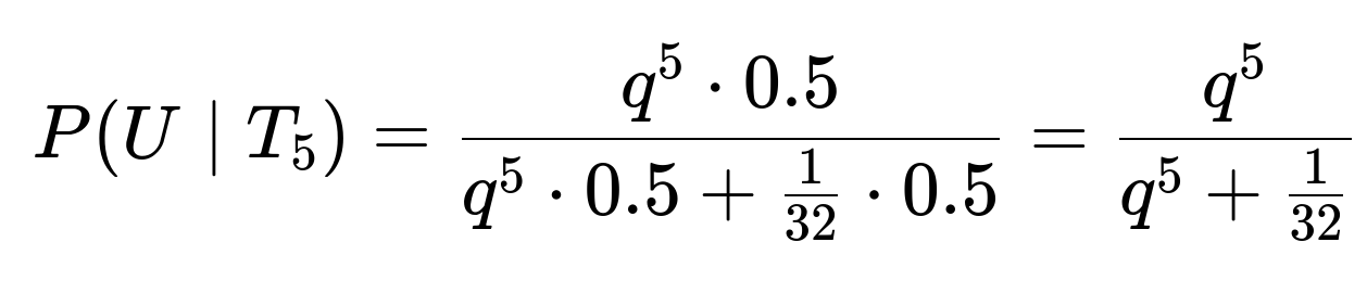
• Hypothesis U: The coin is “unfair,” with probability (q) of landing tails (where (q) is high but not 1).

• Hypothesis F: The coin is “fair,” with probability (0.5) of landing tails.

Seeing 5 tails in a row yields likelihoods:

• (P(T_5 \mid U) = q^5).

• (P(T_5 \mid F) = (0.5)^5 = 1/32).

If the priors are equal, say 0.5 each, then:

If (q) is close to 1 (e.g., 0.99), you get a large fraction. If (q) is only 0.8, then (0.8^5=0.32768). The posterior becomes:

So you’d still be over 91% sure it’s the “unfair” coin, but not nearly as certain as if (q=1).

A pitfall here is that if you incorrectly assume a coin is strictly 0 or 1 probability of tails, you might mis-estimate the posterior. In real life, you’d estimate (q) from multiple flips or from prior knowledge about the manufacturing of trick coins.

Could the presence of an observer’s bias (like “hot hand” fallacy or gambler’s fallacy) affect these judgments?

Yes, cognitive biases can influence how we interpret repeated events. For instance:

• Gambler’s fallacy: People might wrongly expect that after several tails, a head is “due.” They might think the probability of a head is higher than 0.5 because they’ve seen so many tails in a row.

• Hot hand fallacy: They might think if the coin is “on a streak,” it will continue to produce tails.

Both are incorrect if the coin truly has independent flips. But in real life, these biases might cause someone to misjudge or deviate from the Bayesian calculation. The formal Bayesian approach remains correct if the flips are genuinely independent and the coin’s probabilities are known.

A pitfall is letting intuition overshadow correct probability updates. Interviewers might bring up these biases to see if you understand the difference between psychological biases and formal probability theory.

In an engineering setting, how might we use this logic to detect defective components on a production line that always fail a test?

This exact logic generalizes to quality-control settings. Imagine:

• Hypothesis D: A part is defective such that it always fails a certain test.

• Hypothesis G: A part is good (non-defective) with a certain small probability of failing the test (like a fair coin flipping tails).

After you test the part multiple times and see repeated failures, the posterior probability that it is defective grows. Formally, you’d have:

• (P(\text{fail all tests} \mid D) \approx 1).

• (P(\text{fail all tests} \mid G)) could be ((p_{\text{fail}})^n).

Then you use the same Bayesian update to figure out how likely it is you have a defective part. The pitfall is if the tests themselves can be faulty, or if some other factor might cause repeated failures even for a good part. Then you have to model that more precisely.

This scenario also underscores how a single success for a defective part (analogous to flipping a head with a double-tailed coin) would be impossible under the model, thus ruling out the defective hypothesis.

How do we ensure numerical stability if we see a very large number of tails in practice, e.g., 50 tails in a row, when computing the posterior?

When dealing with ((1/2)^{50}), it becomes a very small number ((\approx 8.88 \times 10^{-16})). In a programming environment, you might run into floating-point underflow if you directly compute that value, especially for bigger (n).

To handle this:

• Work in log space. Compute (\log \left(\frac{1}{2}^n\right) = -n \log(2)).

• Then exponentiate only at the end if needed.

Another technique: use specialized libraries (like in Python’s decimal module or in some numeric libraries) that handle small or large numbers more gracefully.

A pitfall is ignoring floating-point limitations and getting 0 due to underflow, which might produce incorrect posterior computations (like a division by 0 scenario). In an interview, discussing log-probabilities is often a good demonstration of numerical best practices in machine learning.

How might we extend the puzzle if the coin can land on its edge with some small probability?

Let’s assume a coin can land on its edge with probability (\epsilon). For a fair coin, maybe it’s (\epsilon\approx 0.01), with the other 0.99 of probability split evenly for heads and tails. For a double-tailed coin, maybe heads is 0, tails is ((1-\epsilon)), and the edge is (\epsilon). Observing 5 tails in a row has different likelihoods:

• (P(T_5 \mid \text{fair with edges}) = (0.495)^5) if heads and tails each get 0.495 probability (since total is (0.99) for heads/tails plus (0.01) for edges).

• (P(T_5 \mid \text{double-tailed with edges}) = (1-\epsilon)^5).

Then the Bayesian posterior formula remains the same in structure, but you’d substitute these new likelihoods.

A subtlety arises if you see an edge in one of your flips. For the double-tailed coin, that’s possible with probability (\epsilon). For the fair coin, also possible with probability (\epsilon). Observing edges complicates the inference but is straightforward to incorporate if you track each outcome type.

A pitfall is failing to account for the possibility of edges and lumping them all in as “tails” or “heads,” thus miscounting your data and miscalculating your posterior.

Could the puzzle be a trick question if we strictly interpret a “fair coin” as having one head and one tail, but the coin is so physically imbalanced that it's effectively not 50-50?

Yes, that is a nuance in language. Often we say “fair coin” to mean it has a 50-50 distribution, but the puzzle statement might literally mean “fair coin” in the sense of having one head side and one tail side but not necessarily 50-50 probabilities in practice. If the puzzle means to interpret “fair coin” as truly 50-50, we proceed with ((1/2)^5). But if it means it just has one head side, one tail side, but physically it might still land tails more or less than half the time, we’d incorporate a bias parameter.

A real-world pitfall is assuming that “one side heads and one side tails” always means exactly 50% probability of landing on tails. In practice, that might not be strictly true, but in puzzle contexts, we usually accept that “fair coin” means 50% chance of tails.

In an interview, always clarify assumptions: “By fair coin, do you explicitly mean 50-50 chance?”

How might the knowledge that you performed a “coin toss selection” instead of a “random coin selection” change the Bayesian prior?

If you had some complicated procedure for picking the coin, say you spun a wheel or you took the first coin from a bag where there are 10 fair coins and 1 double-tailed coin, that changes the prior. For instance, if the bag has 10 fair coins and 1 unfair, then your prior is (\frac{1}{11}) for unfair, (\frac{10}{11}) for fair.

The flipping logic remains the same, but the posterior might be different. For 5 tails, the posterior would be:

$$P(\text{unfair} \mid T_5)

= \frac{1 \times \frac{1}{11}}{1 \times \frac{1}{11} + \frac{1}{32}\times \frac{10}{11}} = \frac{\frac{1}{11}}{\frac{1}{11} + \frac{10}{352}} = \frac{\frac{1}{11}}{\frac{32}{352} + \frac{10}{352}} = \frac{\frac{1}{11}}{\frac{42}{352}} = \frac{32}{33} \times \frac{1}{10}.$$

You’d have to compute that carefully, being sure not to mix up fractions. The essence is that the prior changes everything.

Pitfalls: If the interviewer specifically says you have 10 normal coins and 1 trick coin, and you incorrectly use a prior of 0.5, you’ll get a misleading result. Real-world sampling procedures might not be uniform (some coins might be lost, or the bag might not be thoroughly mixed).

How might we incorporate partial flips (like you tossed the coin but caught it mid-air and only partially saw it) or uncertain outcomes?

In a more general Bayesian model, partial observations can be accounted for by specifying the probability of observing certain partial data given each hypothesis. For example:

• Probability that you see “what looks like a tail” but you’re only 80% sure is actually a tail.

• Probability that you see “unclear result” because the coin fell off the table.

You’d define a likelihood for each partial observation and multiply it into your prior. This is more complicated, but the principle is the same.

A big pitfall is to treat partial or noisy observations as certain outcomes, which leads to incorrect confidence in your posterior. In real applications, distinguishing uncertain from certain observations is essential.

How do we handle a scenario where after seeing 5 tails, we suspect maybe we have a coin that is not necessarily double-tailed, but heavily biased—how do we test that new hypothesis?

This is a problem of “model misspecification.” Initially, we only considered two possibilities: truly fair or truly double-tailed. After seeing the data, we realize another possibility: the coin is biased but not 100% tails.

We then must expand our model set:

• Hypothesis F: Probability of tails = 0.5.

• Hypothesis U: Probability of tails = 1.

• Hypothesis B: Probability of tails = some unknown parameter (\theta) strictly between 0.5 and 1.

Now the updating becomes more intricate because (\theta) might need a prior distribution (like a Beta distribution in a Bayesian approach). You’d update that distribution given the observed flips.

A pitfall is ignoring that new hypothesis entirely, which might lead to an overestimate of the probability that the coin is double-tailed. The data might be explained better by a moderately biased coin. Real interviews often check if you’d question the initial assumptions after observing surprising data.

What if someone else had already flipped the coin 3 times and got 1 head, 2 tails, and then handed it to you. Should you include that data?

From a strict Bayesian standpoint, all available evidence should be included in your posterior. If you trust those 3 flips were done properly and observed reliably, then you incorporate them into your likelihood. Observing 1 head and 2 tails might slightly reduce the posterior that the coin is double-tailed. Then, if you personally flip it 5 times and see 5 tails, you combine all 8 flips of evidence.

Formally, your likelihood for a double-tailed coin for all 8 flips (1 head, 2 tails from them, 5 tails from you) is 0, because you can’t get a head at all. So if the other person’s data is correct, that alone sets the probability of the coin being double-tailed to 0.

A subtlety is deciding how much you trust the other person’s data. If you suspect they might have made a mistake, you might incorporate that uncertainty.

A pitfall is ignoring or discarding relevant data just because you didn’t personally see the flips. In a job interview, showing that you can handle combined evidence is valuable.

If we flip 5 times and get 5 tails, then check the coin physically and see it’s a normal coin with 1 head side and 1 tail side, what does that say about our initial Bayesian calculation?

In that hypothetical scenario, you discovered that the coin is physically not double-tailed. That new observation overrides your previous inference because it’s direct visual evidence. The Bayesian posterior for “unfair coin with 2 tails” becomes 0 if you truly confirm that it has a head side.

It indicates that your initial Bayesian calculation, while correct given the puzzle assumption, was operating under incomplete information. The puzzle’s scenario presumes you can’t examine the coin. Real life rarely matches a puzzle’s constraints perfectly.

One pitfall is failing to revise your beliefs in light of direct contradictory evidence. Another pitfall is ignoring your initial confusion about how you saw 5 tails in a row with a normal coin—maybe it’s still suspiciously biased. But mathematically, if you are 100% sure you physically see 1 head side, you must discard the 2-tailed hypothesis.

How does the result reflect a classic illustration of Bayesian reasoning vs. intuitive reasoning?

This puzzle is a neat demonstration because many might guess something like “Well, 1/32 is pretty small, so it must be definitely the double-tailed coin.” But they might not do the formal calculation. The formal Bayesian update is:

• Weighted by the prior (equal in the puzzle).

• Weighted by the likelihood of the data given each hypothesis.

It yields (\frac{32}{33}). Intuitively, that’s about 97%. It’s not 100%. People’s initial guess might be something like 95% or 99% or 90%. This puzzle shows exactly how to do it precisely.

A pitfall is mixing up p-values with posterior probabilities or conflating “very unlikely event under fair coin” with “impossible event.” Another pitfall is the misconception that “the fair coin can’t give 5 tails.” It can; it’s just less likely. Hence the Bayesian approach is the correct framework for determining how that updated likelihood compares to the alternative.

Could we do maximum likelihood estimation (MLE) to pick which coin it is?

A naive MLE approach would say:

• For the fair coin, the likelihood of 5 tails is ((1/2)^5 = 1/32).

• For the double-tailed coin, the likelihood is 1.

Hence, the double-tailed coin has a higher likelihood, so MLE picks that coin with no notion of prior. If the priors were equal, MLE effectively gives a 100% pick to the double-tailed coin.

However, that ignores the fact that the prior probability might not be 0.5. If the prior for the double-tailed coin were extremely tiny, a pure MLE approach might not be the best final guess. That’s why a Bayesian approach or maximum a posteriori (MAP) approach is often more appropriate.

Pitfall: Relying solely on MLE can lead to ignoring how improbable the double-tailed coin might have been a priori. If the puzzle states the prior is 50-50, MLE and MAP coincide. But if there’s a different prior, MAP might differ from MLE.

If we wanted an unbiased estimator of the probability that the coin is double-tailed, how does that differ from the Bayesian posterior?

An “unbiased estimator” typically refers to an estimator whose expected value matches the true parameter value over repeated sampling. The Bayesian posterior, on the other hand, is a distribution over hypotheses or parameters given your data and prior.

For a discrete hypothesis scenario (fair vs. unfair), the Bayesian posterior is typically the best direct measure of your belief. The concept of an “unbiased estimator” is more relevant to continuous parameter estimation.

Pitfall: Trying to interpret the posterior probability as an unbiased estimator can be conceptually confusing. The posterior is a subjective probability that directly addresses “the probability the coin is double-tailed given the data.” That’s different from a frequentist notion of an unbiased estimator. In an interview, clarifying these differences is important.

How do we confirm if our final numeric result is correct without a calculator or code?

You can simplify as follows:

• Fair coin: Probability of 5 tails = (\tfrac{1}{32}).

• Unfair coin: Probability = 1.

• Priors are 0.5 each.

Hence:

P(unfair | T_5) = (0.5 * 1) / (0.5 * 1 + 0.5 * 1/32) = 0.5 / (0.5 + 0.5 * 1/32) = 0.5 / (0.5 + 0.015625) = 0.5 / 0.515625 = 0.5 / (33/64) = (0.5 * 64) / 33 = 32/33.

Since 1/32 = 0.03125, half of that is 0.015625, add that to 0.5 you get 0.515625, dividing 0.5 by 0.515625 is 0.969..., which is 32/33.

A small pitfall is messing up fraction arithmetic. In a high-pressure interview, double-check.

Another trick: 1/32 = 2/64, so 2/64 ÷ 2 = 1/64, so half of 1/32 is 1/64 = 0.015625. Keeping track carefully helps you avoid basic fraction errors.