
ML Interview Q Series: Calculating Binomial Coin Toss Probabilities using Normal Approximation
Browse all the Probability Interview Questions here.
Question: You conduct 576 fair coin tosses. Without using any calculator, how do you determine the probability of getting at least 312 heads?
Comprehensive Explanation
One standard way to address questions about the probability of obtaining a certain number of heads in a series of fair coin flips is to model the count of heads as a Binomial random variable. For a fair coin, the probability of heads is 0.5, and for 576 independent flips, the number of heads X follows a Binomial distribution with parameters n = 576 and p = 0.5.
The Binomial distribution for the probability of getting exactly k heads out of n trials is

In this formula, n is the total number of coin flips, k is the number of heads, and p = 0.5 for a fair coin. The combination term n choose k is the binomial coefficient that counts the possible ways of choosing k successes out of n trials.
Calculating P(X >= 312) by summing binomial probabilities term by term can be highly cumbersome without a calculator. Instead, the Central Limit Theorem can provide an excellent approximation when n is large. According to the Central Limit Theorem, a Binomial(n, p) distribution can be approximated by a Normal(μ, σ²) distribution with mean μ = n p and variance σ² = n p (1 - p).
For our specific problem:
n = 576
p = 0.5
Mean μ = 576 * 0.5 = 288
Variance = 576 * 0.5 * 0.5 = 144
Standard deviation σ = sqrt(144) = 12
We wish to find P(X >= 312). Using the normal approximation, define the random variable X to be approximately N(μ, σ²). We convert X >= 312 into the standard normal variable Z by subtracting the mean and dividing by the standard deviation.
If we neglect continuity correction for simplicity:

We want P(X >= 312) = P(Z >= (312 - 288)/12). The quantity (312 - 288)/12 = 24/12 = 2. So we have P(Z >= 2).
From standard normal tables (or from well-known approximate values), P(Z >= 2) is around 0.0228. Thus, the probability is approximately 2.28%. This gives us a quick and reasonable estimate for the probability of getting at least 312 heads when flipping a fair coin 576 times.
If we add a continuity correction, we approximate P(X >= 312) by P(X >= 311.5) in the continuous normal distribution. That modifies the Z-value to (311.5 - 288)/12 = 23.5/12 ≈ 1.9583, and that probability would be slightly higher than 0.0228, but the difference is small enough that, for an interview setting without precise tools, 2.3% is a perfectly valid approximate answer.
Many interviewers expect recognition that the normal approximation is valid here because n is large. Additionally, they often look for familiarity with the mean and variance of the Binomial distribution and how to do quick mental approximations or recall standard normal tail probabilities.
How the Continuity Correction Could Impact the Approximation
The continuity correction is used when approximating discrete random variables (like the binomial) with continuous ones (like the normal). For a lower bound event X >= k, you shift to X >= k - 0.5. In this question, it slightly lowers the required Z-value, thereby increasing the probability. The practical difference in large n situations is often small, but it shows thoroughness when you mention it.
Demonstration of the Exact Calculation in Python
Though the question states to solve it without a calculator, in a real-world scenario or if the interviewer allows you to check your approximation, you can use Python or another statistical library. Below is a quick Python code snippet that calculates the exact binomial probability of X >= 312 and compares it to the normal approximation.
import math
from math import comb
from statistics import NormalDist

def binomial_probability_ge(n, p, k):
    # Probability of getting at least k heads out of n
    total_prob = 0.0
    for i in range(k, n + 1):
        total_prob += comb(n, i) * (p**i) * ((1-p)**(n - i))
    return total_prob

n = 576
p = 0.5
k = 312

# Exact Binomial Calculation
exact_prob = binomial_probability_ge(n, p, k)

# Normal Approximation
mu = n * p
sigma = math.sqrt(n * p * (1 - p))
z_value = (k - mu) / sigma
approx_prob = 1 - NormalDist(mu=0, sigma=1).cdf(z_value)

print("Exact Binomial Probability:", exact_prob)
print("Normal Approximation:", approx_prob)
In a genuine interview, you might not run this code, but it demonstrates how you would verify your approximation if needed.
Potential Follow-Up Question: Why Does the Normal Approximation Work Here?
The Central Limit Theorem states that as the number of trials n grows large, the distribution of the sample mean (or equivalently the sum of Bernoulli random variables) approaches a normal distribution. Because each coin flip is a Bernoulli trial, their sum (the total number of heads) is binomially distributed. For large n, the binomial shape becomes nearly symmetric and bell-shaped, which makes the normal approximation quite accurate.
Potential Follow-Up Question: What if the Coin Was Biased?
If p ≠ 0.5, the Binomial(n, p) distribution would still have mean n p and variance n p (1 - p). You would proceed similarly but use the modified mean and variance. The main difference is that the distribution would be skewed if p is not 0.5, so sometimes a normal approximation may be slightly less accurate when p is close to 0 or 1. For moderate p values away from the extremes and large n, it remains a good approximation.
Potential Follow-Up Question: Are There Other Approximations for Binomial?
For large n but with p potentially very small or large, the Poisson approximation can be used when n p is of moderate size and n is large, or the Chernoff bound can give a bound on the tail probabilities. The choice depends on the problem’s specifics and what form of approximation is most suitable.
Potential Follow-Up Question: What If We Needed More Precision Without a Calculator?
One possibility is to use a refined normal table or certain inequalities (like Hoeffding’s or Chernoff’s bounds). Alternatively, for smaller n, you can use the symmetry of the binomial distribution around its mean when p = 0.5. Also, if you are careful with partial sums of binomial probabilities, you might apply combinatorial identities, but this is rarely done in practice for large n without computational tools.
Below are additional follow-up questions
How does the normal approximation behave in borderline cases, for example when k is very close to n/2 or very far from n/2?
The normal approximation performs best around the mean of the binomial distribution—particularly when p = 0.5—because the distribution is most symmetrical. When k is extremely close to the mean (for instance, 288 out of 576) the approximation is usually excellent. However, if k is very far from the mean (either very large or very small), the tail behavior of the binomial can differ notably from that of the normal distribution. This can lead to a less accurate approximation in the extreme tails. One way to mitigate inaccuracy around boundaries is to use continuity corrections, or more advanced bounds like Chernoff bounds for large deviations.
What if the event we are examining is something like flipping at least 576 heads in 576 trials (i.e., all heads)? Would the normal approximation still be relevant?
The normal approximation is weakest in the extreme tails of the distribution, such as the event of getting all heads or zero heads. In these cases, the binomial probabilities are often so small that the normal approximation might give you a probability effectively zero even if the exact binomial formula would yield a tiny (but nonzero) probability. In practical terms, when you see events like “all heads,” it is better to use the exact binomial formula or a specialized bound because the normal approximation is not well-suited for extremely rare events.
How do you handle or interpret dependencies between coin flips if they are not truly independent?
Real-world scenarios might introduce dependencies (e.g., if the coin flips were correlated for some reason). In such cases, the binomial model no longer holds strictly since the fundamental assumption of independent Bernoulli trials is violated. You might model correlated outcomes with other distributions or use more general methods (Markov chain modeling, copulas, or other joint distribution approaches). One must then either derive or approximate the joint probability distribution of heads. Additionally, the Central Limit Theorem can extend to certain correlated processes (under suitable mixing or weak dependence conditions), but checking the assumptions is crucial to ensure the approximation remains valid.
How would you calculate a p-value in a hypothesis testing framework for “at least 312 heads in 576 flips” if the null hypothesis is that the coin is fair?
You would treat the number of heads as a test statistic under H0: p = 0.5. The p-value is P(X >= 312) under the binomial distribution with n = 576, p = 0.5. If you had a table or standard normal distribution knowledge, you would do the normal approximation (with continuity correction) to get an approximate p-value. In formal hypothesis testing, if that p-value is below a chosen significance level (like 0.05), you would reject H0. For large n, the normal approximation is standard. In a real analysis setting or with computational tools, you could use the exact binomial calculation for a precise value.
Could you explain when to use Chernoff bounds or other large deviation inequalities?
Chernoff bounds or other concentration inequalities (like Hoeffding’s or Bernstein’s bounds) can provide strong tail probability bounds for sums of independent Bernoulli trials. They can be particularly useful when you need a guaranteed upper bound on the probability of deviating from the mean by a certain margin, without having to rely on the normal approximation. For a binomial random variable X with parameters n and p, Chernoff bounds say (for X >= (p + δ)n):
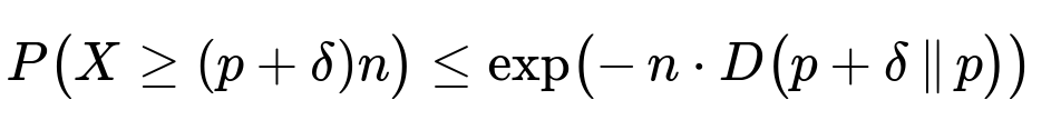
where D(a || b) = a ln(a/b) + (1-a) ln((1-a)/(1-b)) is the Kullback–Leibler divergence (in text form). This bound is exact in the sense of it does not require continuity correction and typically provides a tighter result than a simple Chebyshev or normal approximation, especially for the tail events that are farther from the mean.
What is the impact of partial or incomplete data, for instance, if we only observe a subset of the flips?
If the data about coin flips is incomplete or censored (maybe some flips weren’t recorded properly), the straightforward application of the binomial distribution no longer holds. You might need to use missing data techniques (such as expectation-maximization if you had partial knowledge of p) or treat unobserved flips as random variables themselves. The result is that your variance in estimating the probability of “at least k heads” would increase because you have less information. If possible, you’d incorporate prior knowledge about p or the distribution of missingness to refine your estimates.
How do we handle a scenario where the coin changes its bias over time?
If the coin’s probability of heads, p, shifts with each flip (for example, due to mechanical wear on the coin or environmental changes), then the simple Binomial(n, p) model is invalid because p is no longer constant. One might model the sequence of coin flips with a time-varying p_i for the i-th flip, leading to a Poisson binomial distribution, which is the distribution of a sum of independent Bernoulli trials that have different success probabilities. Approximations like the normal distribution can still apply under certain conditions (e.g., if the p_i’s cluster around some mean or if you can prove a general version of the Central Limit Theorem for non-identical distributions). However, the calculations or approximations become more involved, and exact formulae for Poisson binomial probabilities might need specialized algorithms.
How would you approach computing the probability if the number of flips was extremely large, such as millions or billions of flips?
For extremely large n (like millions of flips), direct binomial calculations are computationally impossible in a naive manner. Even normal approximation might require caution because if n is very large and p is not 0.5, the distribution can be highly skewed. Nevertheless, the Central Limit Theorem generally gives a good first approximation. In cases where p is close to 0 or close to 1, the Poisson approximation (when p is small) or other specialized approximations (when p is near 1) might be more accurate. Parallelizable Monte Carlo simulations are also common: simulate many sequences or use advanced variance reduction techniques. For large-scale real-world scenarios (like streaming data in web applications), incremental updates to approximate the distribution can be done with streaming algorithms.
Can quantile-based approximations be used when calculating this probability?
Yes. Instead of focusing on the distribution’s tail via integrals or sums, sometimes you approximate the relevant quantiles directly. For instance, one might use the inverse normal approximation to find the z-quantile and convert it back to the binomial scale. These techniques rely on the same central limit logic but can be simpler if you only need an approximate boundary. They may, however, miss subtle details of the discrete nature of the binomial distribution unless you include a continuity correction.
How might we interpret or handle the event of “exactly 312 heads” rather than “at least 312 heads”?
For exactly 312 heads, the binomial probability is P(X = 312). With n = 576, p = 0.5, that term by itself can be computed with the binomial formula or approximated by the height of the normal distribution near its mean—though you would typically do P(311.5 < X < 312.5) in the normal domain with a continuity correction. The probability of exactly k events in a large n scenario is roughly the difference between the normal CDF at k+0.5 and k−0.5. For central values, it usually matches quite well, but for extreme k values, the normal approach can underestimate or overestimate the exact discrete probability.
Under what conditions would a skewed distribution demand more caution in applying the normal approximation?
When p is significantly different from 0.5 (e.g., p = 0.01 or p = 0.99), the binomial distribution becomes highly skewed. The normal approximation can still be used if n is large enough that both n p and n (1 − p) are comfortably above 10 (a common rule of thumb). However, the more extreme the skew, the more you must rely on continuity corrections or alternative approximations (e.g., Poisson for small p, or approximations around 1 − p for large p) to maintain acceptable accuracy.
What if we’re not just interested in “at least 312 heads” but the entire distribution of heads?
You might be interested in the probability mass function (PMF), cumulative distribution function (CDF), or other statistics (like percentiles). In such cases: • You could build the entire binomial PMF by enumerating k from 0 to n, though it can be huge for large n. • Use normal approximation to build a continuous approximation to the PMF or CDF. • Implement more advanced methods like the incomplete beta function for the CDF of a binomial or rely on specialized algorithms for computing binomial distribution probabilities efficiently (e.g., dynamic programming if n is not too large, or log-space summation for stability).
What happens if the sampling process is adaptive? For instance, we flip until we see a certain outcome and then change the procedure?
In adaptive or sequential experiments, the number of trials might not be fixed in advance, or p might be adaptively modified. Then your final distribution for the number of heads is not purely binomial. Methods like Wald’s Sequential Probability Ratio Test or Bayesian updating might be relevant. The design of the experiment and the stopping rule strongly affect the final distribution of outcomes. For instance, if you flip until you see 312 heads, the distribution for the total number of flips is negative binomial-like rather than binomial.
How could you construct a confidence interval for p once you observe 312 heads out of 576 trials?
A typical approach is to use the Clopper-Pearson interval, which is an exact method for binomial confidence intervals. Approximate methods include the Wald interval (p-hat ± z * sqrt(p-hat(1−p-hat)/n)), Wilson score interval, or Agresti–Coull interval. For large n, the normal-based interval is often fine, but for smaller samples or extreme p values, more accurate intervals like Wilson or Clopper-Pearson are recommended. If you see 312 heads out of 576, the point estimate p-hat is 312/576. You’d then plug that into your chosen interval formula. For large n, the difference among intervals is small, but in a high-stakes application, it’s important to choose an interval that properly handles tail probabilities and small or large values of p.
What practical limitations might arise if we tried to generate confidence bounds for “at least 312 heads” while the experiment was ongoing?
In real time, you might want to see if the threshold of 312 heads is likely to be met or not before completing all flips. You could use a predictive distribution to estimate how many heads you’ll end up with, given the results so far. Bayesian methods are especially convenient for this, as you can maintain a posterior over p and project forward. Alternatively, frequentist approaches might use interim analyses but risk inflating Type I errors if you repeatedly peek at the data. Handling these practicalities demands advanced knowledge of sequential testing or online algorithms.
Could results be skewed if the coin’s outcomes are physically or systematically biased during the flipping process (e.g., “thumb flips” or not flipping the coin enough rotations)?
Absolutely. The simplest binomial model with p = 0.5 assumes an idealized fair coin and independent, unbiased flips. However, experimental or mechanical factors can change p in subtle ways. Studies have shown that certain ways of flipping a coin can bias the outcome slightly. In the real world, if the flipping mechanism is not random enough, the true p can deviate from 0.5, or the flips might not be i.i.d. For rigorous analysis, one must ensure that the flipping process is indeed random. Otherwise, the entire binomial assumption is questionable, and you would have to measure or estimate the actual bias introduced by the flipping methodology.