
ML Interview Q Series: Calculating Tree Failure Probability via Total Probability Law and Hypergeometric Sampling.

Browse all the Probability Interview Questions here.
You have bought 10 young beech trees. They come from a garden center and were randomly chosen from a collection of 100 trees consisting of 50 trees from tree-nurseryman A and 50 trees from tree-nurseryman B. Ten percent of the trees from tree-nurseryman A and five percent of the trees from tree-nurseryman B do not grow well. What is the probability that no more than one of your ten trees will not grow well?
Short Compact solution
We let k be the number of trees out of the 10 that come from nurseryman A (and thus 10−k come from B). The probability of having exactly k trees from A is:

We then compute the probability that no more than one of the ten trees fails to grow well, given that k are from A. Denote this event by E. The conditional probability P(E | B_k) is the sum of:
The probability that none of the 10 fail: (0.90^k)(0.95^(10−k))
The probability exactly 1 from A fails: (k choose 1)0.10(0.90^(k−1))*(0.95^(10−k))
The probability exactly 1 from B fails: ((10−k) choose 1)0.05(0.95^(9−k))*(0.90^k)
Hence:


Plugging in the values yields:
P(E) ≈ 0.8243.
Comprehensive Explanation
Understanding the setup
We randomly select 10 beech trees from a total of 100. Half of these 100 trees (50) are from nurseryman A and half (50) are from nurseryman B. A tree from A has a 10% chance (0.10) of failing to grow well; a tree from B has a 5% chance (0.05) of failing.
We want the probability that among the 10 chosen trees, at most one will fail to grow well. Because the selection is random, the number of trees k coming from A (and thus 10−k from B) follows a hypergeometric distribution.
Hypergeometric selection probability
The probability that exactly k of the chosen 10 trees come from the 50 trees of nurseryman A is given by choosing k out of A’s 50 trees and 10−k out of B’s 50 trees, divided by all ways to choose 10 out of 100:
P(B_k) = ( (50 choose k) * (50 choose 10−k) ) / ( (100 choose 10) ).
This captures the randomness of how many A-trees (k) you end up with in your set of 10.
Conditional probability: no more than one failure
Given that exactly k trees come from A, we know those k trees each fail with probability 0.10, and the remaining 10−k trees each fail with probability 0.05. We then consider the event E: “no more than one fails.”
Probability that none fail: all k from A must succeed (each with probability 0.90) and all 10−k from B must succeed (each with probability 0.95). Multiplying these yields 0.90^k * 0.95^(10−k).
Probability that exactly 1 fails:
That 1 failure could come from the A-subset (k choose 1) ways, with fail probability 0.10 and success probability 0.90^(k−1) for the other A trees, and 0.95^(10−k) for all B trees.
Or that 1 failure could come from the B-subset ((10−k) choose 1) ways, with fail probability 0.05, success probability 0.95^( (10−k)−1 ), and 0.90^k for all A trees.
Hence,
P(E | B_k) = (0.90^k)(0.95^(10−k)) + (k choose 1)0.10(0.90^(k−1))(0.95^(10−k)) + ((10−k) choose 1)0.05(0.95^(9−k))(0.90^k).
Total probability
We then weight P(E | B_k) by the probability P(B_k) that there are exactly k A-trees among the chosen 10 and sum over k=0 to 10:
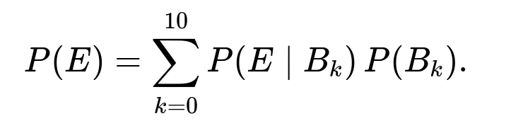
Computing this sum yields approximately 0.8243.
Why this approach works
We separate the problem into cases based on how many A-trees (and B-trees) are chosen, then compute the probability of at most one failure within each case. Because each case occurs with probability P(B_k), we weight that case’s success probability by P(B_k). This is a classic application of the law of total probability, where partitioning the sample space according to how many A-trees are selected simplifies the analysis.
Additional Question: Could we have modeled this problem using a direct combinatorial approach instead?
Yes, but it would be more complicated. One could attempt to directly count the ways in which 0 or 1 tree out of the 10 fails, accounting for the probabilities 0.10 and 0.05 for different subsets. This direct approach would involve splitting into numerous combinatorial scenarios: how many fail from A vs. from B and how many are chosen from each group. The hypergeometric condition on k from A (and 10−k from B) is what naturally leads us to break it down into simpler subproblems.
Additional Question: How can we implement this calculation in Python?
A straightforward way is to implement each piece and sum them up. For instance:
import math

def choose(n, r):
    return math.comb(n, r)

p_E = 0.0
for k in range(11):  # k goes from 0 to 10
    # Probability k come from A
    p_Bk = (choose(50, k) * choose(50, 10 - k)) / choose(100, 10)

    # Probability no more than one fails
    # none fail:
    p_none_fail = (0.90**k)*(0.95**(10 - k))

    # exactly 1 fails in A:
    if k >= 1:
        p_one_fail_A = choose(k, 1)*0.10*(0.90**(k-1))*(0.95**(10 - k))
    else:
        p_one_fail_A = 0.0

    # exactly 1 fails in B:
    if (10 - k) >= 1:
        p_one_fail_B = choose(10 - k, 1)*0.05*(0.95**((10 - k) - 1))*(0.90**k)
    else:
        p_one_fail_B = 0.0

    p_E_given_Bk = p_none_fail + p_one_fail_A + p_one_fail_B
    p_E += p_E_given_Bk * p_Bk

print(p_E)
This code enumerates k=0..10, computes the probability P(B_k), and then calculates P(E | B_k), finally summing up for the total P(E).
Additional Question: What if the failure probabilities were different for each tree, not just grouped by nurseryman?
If every tree had a distinct probability of failing, we could not simply group them by A and B. We would need to consider the exact probability that each chosen tree fails and then count or sum over all subsets of trees that fail. In practice, we might do a direct calculation with repeated sums or a dynamic programming approach to handle up to 10 trees. The partitioning strategy with B_k would no longer suffice if each tree is truly unique in its failure probability.
Additional Question: How might this appear in a real-world setting?
In horticulture or agriculture, it is common for different suppliers (nurseries) to have slightly different standards or success rates due to factors like seed quality, rootstock health, or storage conditions. One might want to estimate the chance that a landscaping project meets quality requirements (for instance, no more than 10% of trees fail). The approach used here can generalize to other domains: any time you have multiple subpopulations (e.g., from different suppliers) and randomly draw from the combined population, you can use the law of total probability, conditional on how many items come from each subpopulation, to compute an overall success/failure probability.
Below are additional follow-up questions
How would the answer change if we attempted a binomial approximation instead of the exact hypergeometric approach?
A binomial approximation might be used if the population is large compared to the sample size. We would say each tree has some “average” probability of failing, and then we treat the 10 trees as identically distributed. But here, because there are exactly 50 trees from A and 50 from B in the entire population, the hypergeometric nature is quite important. If the population was extremely large (for example, 50,000 from A and 50,000 from B) and we still only sampled 10, the proportion of A vs. B in our sample would be almost constant (close to 50% of each). Then one might approximate k as binomial with parameter p=0.5. In that case, the chance of failure from A vs. B would be assigned from separate Bernoulli processes. That said, the direct binomial approach would ignore the slight variability in the sample composition of A vs. B. Pitfall: Using the binomial approximation can overlook small but potentially important differences caused by exact constraints. When the population is not extremely large relative to the sample, or when k is constrained (like half from A and half from B is not guaranteed, but the population ratio is exactly 1:1), ignoring the hypergeometric structure can introduce inaccuracies.
If the proportions from A and B were not equal (e.g., 60 from A and 40 from B), how would we handle it?
We would modify the probability P(B_k) of drawing k trees from A out of 10. Specifically, we replace the numbers in the hypergeometric formula: choose(60, k)*choose(40, 10−k) / choose(100, 10). The rest of the logic remains unchanged. We would still compute a conditional probability of “at most one failure” given k A-trees and 10−k B-trees, and then apply the law of total probability. Pitfall: Forgetting to update the hypergeometric distribution for the new ratio of A vs. B leads to an incorrect result. Always ensure that the formula for P(B_k) matches the actual count of A-trees and B-trees in the total population.
What if the outcome of one tree might depend on the outcomes of others (i.e., there is correlation in their failures)?
Our solution implicitly assumes each tree’s fate is independent, given that it is from A or B. In reality, plant failures can sometimes be correlated (e.g., if all trees are planted in the same poor soil conditions, multiple might fail). If there is correlation, we cannot simply multiply individual probabilities like (0.90^k) or (0.95^(10−k)) to get joint probabilities. We would need a joint probability model capturing that dependence (for example, a correlation parameter or a more complex model). Pitfall: Blindly applying the multiplication rule in the presence of correlation can seriously misrepresent the true risk of multiple failures. Real-world horticultural projects often face similar environmental conditions for all seedlings, so the chance of group failures might be higher than predicted by an independent model.
How does the approach change if we needed the probability that at most two (or at most three) trees fail?
The same law of total probability applies, but we adjust P(E | B_k). Instead of summing the probabilities of “0 or 1 failure,” we would sum up the probabilities of “0, 1, or 2 failures” (or further up to 3). For example, for at most two failures, we would calculate:
Probability of 0 failures
Probability of exactly 1 failure
Probability of exactly 2 failures all conditioned on B_k, and then sum them. Finally, we multiply by P(B_k) and sum over k=0..10. Pitfall: If you only look at partial sums or forget one of the cases, you incorrectly calculate the probability. Carefully enumerate all relevant failure counts to avoid missing a scenario.
Could we use a normal approximation for large sample sizes?
If the sample size is large, and the population also large, some might consider a normal approximation to the distribution of the total number of failures. One approach is to use a hypergeometric-to-binomial approximation, then approximate that binomial by a normal distribution with mean np and variance np(1−p). However, with only 10 trees sampled, a normal approximation is not appropriate: the distribution is discrete and heavily skewed. Pitfall: The normal approximation can be very inaccurate with small n (like 10) or with success probabilities near 0 or 1. You need sufficiently large n for the central limit theorem to help. In this problem, n=10 is too small for a reliable normal approximation.
What if the probability of failure for nurseryman A or B is not known exactly but has its own uncertainty?
This introduces a Bayesian perspective or a hierarchical model. We would treat the failure probability for A as a random variable itself, say p_A, with a prior distribution, and similarly for B. Then we would integrate out that uncertainty when computing the probability of “no more than one fails.” That might involve using beta prior distributions for p_A and p_B and updating them with observational data. Pitfall: Failing to account for uncertain or imprecise knowledge of p_A or p_B can lead to overconfidence in the final probability. In real scenarios, we often estimate these probabilities from historical data, which introduces parameter estimation error.
How might extreme edge cases (e.g., all 10 trees come from A or all 10 from B) affect the result?
Although rare, it is possible for k=10 (all from A) or k=0 (all from B). We account for these in our sum from k=0 to k=10. If someone mistakenly only sums from k=1 to k=9, then the probability of the extreme cases is ignored and the result is incomplete. Pitfall: Omission of edge cases can give an incomplete total probability. Even if the chance of drawing all from A (or all from B) is small, it must be included for mathematical correctness.
In practice, how would we verify or validate that the probability of 0.8243 is realistic?
One way is to look at real data: track a large number of 10-tree purchases from this mixed population, measure how many times at most one fails, and estimate the empirical frequency. Compare that frequency with the theoretical 0.8243. If the empirical frequency is close to 0.8243, then our model is validated. If not, we investigate assumptions (e.g., independence, correct p_A/p_B, or the hypergeometric selection). Pitfall: If real data systematically deviate from our predicted probability, it might indicate hidden factors such as correlation, misidentified failure probabilities, or population changes over time (e.g., the ratio of A to B is no longer exactly 50:50).