
ML Interview Q Series: Calculating Median Probability for Uniform Variables using the Binomial Distribution.

Browse all the Probability Interview Questions here.
Suppose we have three independent random variables, each uniformly distributed over [0, 4]. What is the probability that the median among these three values is greater than 3?
Comprehensive Explanation
One way to understand the event “median > 3” among three identically distributed uniform(0,4) random variables is to note that for the median (the second-largest value) to exceed 3, at least two out of the three values must lie above 3. Because each random variable is uniform(0,4), the probability that any one of them is greater than 3 is 1/4, and the probability that any one is at most 3 is 3/4.
To make it more explicit, let p = Probability(X > 3) for X ~ uniform(0,4). Then p = 1/4. The median exceeding 3 is equivalent to having at least two variables greater than 3. We can thus calculate this probability using the Binomial distribution formula for k successes in 3 trials, where success probability p = 1/4:
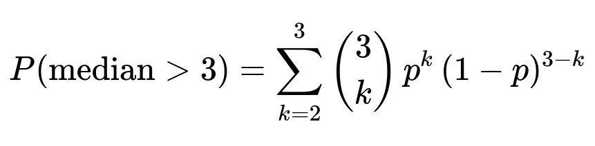
Here, k indicates the number of random variables exceeding 3, and p = 1/4. Substituting p = 1/4 and (1-p) = 3/4:
Probability exactly 2 variables exceed 3: 3 * (1/4)^2 * (3/4)
Probability exactly 3 variables exceed 3: 1 * (1/4)^3
Combining both:
3 * (1/4)^2 * (3/4) + (1/4)^3 = 3 * (1/16) * (3/4) + 1/64 = 9/64 + 1/64 = 10/64 = 5/32
Hence, the probability that the median of three i.i.d. uniform(0,4) random variables is greater than 3 is 5/32, which is approximately 0.15625.
Simulation in Python
Below is an illustrative simulation. We generate three samples from uniform(0,4), compute the median, and see how often it exceeds 3. This code is not a formal proof but serves as a helpful approximation and validation:
import numpy as np

np.random.seed(42)
N = 10_000_000  # number of trials
data = np.random.uniform(0, 4, (N, 3))
medians = np.median(data, axis=1)
estimate = np.mean(medians > 3)
print("Estimated Probability:", estimate)
As N becomes large, estimate should get closer to the theoretical value of 5/32.
Why the Binomial Approach Works
Because the variables are independent, each has an identical probability of exceeding 3. The median of three variables is the second-largest observation. For this to exceed 3, at least two out of the three must exceed 3. Hence we can frame it as a “number of successes in 3 independent trials” problem, with success defined as “value > 3.”
Potential Alternative Methods
One could also perform a direct integration approach over the joint density of three uniform(0,4) variables and then integrate the region that satisfies “median > 3.” However, the combinatorial Binomial shortcut is much simpler in this special case.
Follow-up Questions
How would the calculation differ if the distribution were not uniform?
If the distribution is not uniform(0,4), we need to know p = Probability(X > 3) under the new distribution. The only change in the formula is the value of p. For a general continuous distribution F(x), p = 1 - F(3). The Binomial-based reasoning (at least two out of three exceed 3) remains valid as long as the variables are independent and identically distributed.
Would the result change if we asked for the mean instead of the median?
Yes. The probability that the mean exceeds 3 is different and typically requires integrating the joint density over the subset of the space where X1 + X2 + X3 > 9 (since the average would be (X1 + X2 + X3)/3). For a uniform(0,4) distribution, this region is more complex to handle combinatorially, so we would typically do a triple integral or a simulation approach.
What if the question asked about the maximum or minimum exceeding some threshold?
The probability that the maximum of the three variables exceeds a threshold t is simpler to compute: it is 1 minus the probability that all three are less than or equal to t. Similarly, the probability the minimum exceeds t is the probability all three exceed t. For the median, we need at least two variables to exceed t, which is why the Binomial approach with k = 2 or 3 works.
How can this logic extend to more than three variables?
For n variables, the median is the (n+1)/2-th largest for odd n. You would need at least (n+1)/2 variables above the threshold for the median to exceed that threshold. Then you sum the Binomial probabilities for k from (n+1)/2 up to n, each with success probability p. The same principle applies for even n, but the median definition typically involves averaging the two middle values. The approach becomes slightly more involved, though the Binomial logic still helps for bounding or exact computations in certain interpretations.
Could this create issues in real data scenarios?
Real-world data might not follow a perfect uniform distribution. Dependencies between data points can also break the simple Binomial assumption. Outliers and data shifts can further complicate the interpretation of “median > 3.” In practice, thorough statistical tests, robust distribution checks, and domain knowledge are essential to ensure the assumptions align well with real data.
Below are additional follow-up questions
What if we interpret “median > 3” under a conditional sampling scenario?
One subtle scenario arises if we impose a condition on the sample space, such as discarding any sample set where the maximum (or minimum) is below (or above) a certain threshold. This changes the distribution from unconditional uniform(0,4) to a conditional one, which alters the probability of “median > 3.” For example, if we only keep samples where at least one observation is above 1, the probability changes because we are now sampling from a smaller region of the original distribution. • Practical Pitfall: In real experiments, data might get censored or truncated (e.g., device measurement limitations). If we do not account for this truncation, our estimated probability can be biased. • Deep Explanation: The unconditional probability of the median being above 3 might no longer hold once you restrict the domain. One would have to explicitly recast the random variables with the conditional distribution, re-calculate p = Probability(X > 3) under this new distribution, and then proceed with the Binomial logic if independence is still assumed.
How does sampling error affect our probability estimate in a real-world experiment?
Even though the true theoretical probability is 5/32, in a practical scenario with finite samples, the estimated probability will vary. • Potential Pitfalls: – Small Sample Size: With few experiments, the proportion of medians above 3 may deviate significantly from 5/32. – Statistical Fluctuations: If there is any slight correlation in measurements (e.g., sensor drift that causes correlated readings), the assumption of independence is violated, leading to possible misestimation. • Deep Explanation: If the real setting only allows you to collect, say, 50 triplets of observations, the fraction of medians above 3 could be quite different. Confidence intervals around that fraction are necessary to quantify how much sampling error might impact the result.
Could ties influence the calculation in discrete or coarsely measured data?
In continuous uniform distributions, ties have probability zero. But in discrete-valued or coarsely quantized data, ties can happen with non-trivial probability. If measurements can only take integer values between 0 and 4, the event “median > 3” has to carefully handle cases where two or three values are exactly 3. • Key Pitfall: For discrete or quantized data, one might incorrectly apply the continuous distribution logic. In reality, the median in the presence of ties might behave differently (e.g., if all three values are exactly 3, the median is 3, not above 3). • Deep Explanation: With discrete data, you would need a counting or combinatorial approach that includes tie scenarios. The probabilities of X > 3, X = 3, and X < 3 would each be computed based on discrete mass function values, and you’d compute the probability that at least two samples exceed 3 (strictly greater) when possible.
How does the probability of the median exceeding 3 change if the variables are independent but not identically distributed?
The Binomial argument hinges on the events “X > 3” having the same probability p for each of the three variables. If they are independent but each has a different distribution, the probability of “X1 > 3,” “X2 > 3,” and “X3 > 3” might differ. • Pitfalls: – Mismatched Distributions: If one variable is uniform(0,2) while another is uniform(2,4), the distribution of their medians can shift dramatically. – Incorrectly Applying the Binomial: You cannot just assume a single p and multiply. You would need to carefully sum all combinations where at least two variables exceed 3, each with its own probability. • Deep Explanation: In that scenario, let p1 = Probability(X1 > 3), p2 = Probability(X2 > 3), p3 = Probability(X3 > 3). The probability “median > 3” then equals Probability(at least two exceed 3) = sum of probabilities of exactly two exceed 3 plus probability all three exceed 3, each combination involving p1, p2, p3, and the appropriate factors for (1-pi).
Would the question change if the measurement scale was from 0 to 4 but the phenomenon truly extends beyond these bounds?
Sometimes, we measure a quantity on an instrument that can only report 0 to 4, but the true range is broader. For instance, maybe anything above 4 saturates the sensor at 4. • Pitfalls: – Saturation: Real sensor data might cap at 4, making the distribution not truly uniform(0,4). High values get clipped to 4, so the effective distribution is no longer uniform. – Misleading Probability of “> 3”: If many real values are actually > 4 but read as 4, that lumps all large values into one category, artificially boosting Probability(X > 3) in measured data. • Deep Explanation: In such saturated cases, the nominal uniform(0,4) assumption breaks. A more accurate approach would involve calibrating the sensor or modeling the saturation effect. Otherwise, your estimate of the median surpassing 3 might be inflated or deflated relative to the true phenomenon.
What happens if the question is about the conditional probability that the median is above 3 given that the maximum is above 3?
This introduces a dependence in the variables we look at. The event “maximum > 3” certainly influences the likelihood that the median is above 3. • Key Pitfall: If you simply take the unconditional result 5/32 and try to adjust after the fact that the maximum is above 3, you could be double-counting or ignoring dependencies among the three random variables. • Deep Explanation: The probability that the median is above 3 given that the maximum is above 3 is the fraction of those outcomes where all three are above 3 plus those outcomes where exactly two are above 3 but at least one is above 3 (which is guaranteed by the condition). One must carefully condition on the subset of outcomes for which max(X1, X2, X3) > 3, then calculate how many in that subset have at least two observations above 3.
How does the question extend to comparing two medians from different samples?
Another extension is if we collect three uniform(0,4) variables from one process and three uniform(0,4) variables from another process, and ask, “What is the probability that the median of the first group exceeds the median of the second group?” • Pitfalls: – Overlooking Joint Distribution: You now have six total random variables. Assuming independence across all six, you can write a probability expression that the median of the first trio is above the median of the second trio. This quickly becomes more complex, especially if the distributions differ or if the pairs are correlated. – Edge Cases: If the two processes differ slightly (e.g., one uniform(1,5) and the other uniform(0,4)), the distributions shift. • Deep Explanation: To approach this carefully, you would need to compute or approximate the distribution of each median, then integrate over the two-dimensional space where median1 > median2. Simulation is often simpler in real applications, or you might use known distributions of the order statistics.
What if we seek not just a probability but a full distribution of the median?
Sometimes the question extends beyond “Is the median above 3?” to “What is the distribution function (CDF or PDF) of the median?” • Potential Pitfall: One might think the median is uniform(0,4) as well, which is incorrect. The median of three uniform(0,4) variables has its own distribution. • Deep Explanation: For three i.i.d. continuous random variables, the PDF of the middle order statistic can be derived by enumerating the ways one variable can be the middle value. The distribution is typically found using the formula for the k-th order statistic of n i.i.d. random variables. In the case n=3 and k=2, one can compute that PDF or CDF explicitly. This is more involved but is well-documented in order statistics theory.
Is there a closed-form expression for the expected value of the median, and how might it compare to the question about the probability the median exceeds a certain threshold?
The expected value of the median for three uniform(0,4) variables is not equal to the midpoint of 0 and 4 (which is 2). Instead, it is typically somewhere in the middle but can be derived from the distribution of the second order statistic. • Pitfalls: – Confusing the median of the sample with the mean of the distribution: For uniform(0,4), the mean is 2, but the expected sample median of three draws is also 2. In general, for uniform(0,1) with three draws, the expected median is 1/2. For uniform(0,4), by linear scaling, it becomes 2. – Over-interpreting: While the expected median is 2, that does not immediately tell you the probability that the median exceeds 3. • Deep Explanation: The fact that the mean of uniform(0,4) is 2 and the expected median for three draws is also 2 is consistent because for symmetrical distributions, the expected median is indeed the central point. However, the probability that the median is beyond some threshold must still be computed using the Binomial or order-statistics approach.
Are there scenarios where numerical instability or floating-point precision could affect the computation?
If we were implementing a high-performance Monte Carlo simulation, floating-point precision might cause extremely small probabilities to underflow or large counts to overflow. • Pitfalls: – Running Sum Issues: If you accumulate probabilities in a naive floating-point manner, you might lose precision for large sample sizes. – Using Single Precision Instead of Double Precision: This might create noticeable discrepancies in the estimated probability. • Deep Explanation: Good numerical libraries in Python, C++, or other languages typically mitigate these issues by using double precision. For extremely large sample sizes, special techniques (like Kahan summation or higher-precision libraries) can be used to handle minute probabilities or tiny differences more reliably.
What if in practice the threshold changes dynamically, e.g., from 3 to some function of the observed samples?
A more dynamic question might be: “What is the probability that the median exceeds Q3 + 1,” where Q3 is the third quartile observed in previous data. This complicates the problem because the threshold is no longer a fixed constant but a statistic that depends on data. • Pitfall: – Circular Reasoning: If you use sample data to define the threshold, and then try to compute a probability that the median of a new set will exceed that threshold, you must carefully define whether that threshold is known (treated as a constant) or random. – Overfitting: Using a threshold derived from the same distribution might not be stable if the data sample used to define the threshold is small or unrepresentative. • Deep Explanation: The approach to computing the probability the median surpasses a random threshold Q3 requires joint consideration of the distribution of Q3 and the distribution of the new median. This might involve hierarchical modeling, Bayesian techniques, or empirical bootstrapping methods.
What if, instead of using the strict median, we have a weighted median?
Sometimes we use a weighted median where each value is assigned a different weight. If we have three draws, but each draw is not equally influential, the “middle” by cumulative weight might shift. • Pitfall: – Unclear Definition: Weighted median with just three points is not necessarily the middle value in the usual sense. If one variable has half the total weight alone, it can heavily dominate the “median.” – Implementation Details: In code or in a theoretical formula, you have to carefully handle how weights are assigned and sorted. • Deep Explanation: For three i.i.d. random variables but with different weights, the concept of “median > 3” might become “the point at which half the total weight is to the left.” If one point has weight 0.6 and the other two each have 0.2, you need to check how the realized values line up in sorted order and then see which value crosses the 0.5 total weight boundary.