
ML Interview Q Series: Calculating the Expected Number of Highway Car Clumps Using Recursion.

Browse all the Probability Interview Questions here.
Suppose (N) cars start in a random order along an infinitely long one-lane highway. They are all going at different but constant speeds and cannot pass each other. If a faster car ends up behind a slower car, it must reduce its speed to match the slower car. Eventually, the cars will form one or more clumps (traffic jams). Use a recursion to find the expected number of clumps of cars.
Short Compact solution
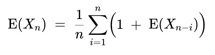
We denote by (X_n) the number of clumps that form when there are (n) cars. Let (Y) be the position (in the order from front to back) of the slowest car. Conditional on (Y = i), the slowest car “splits” the configuration so that the expected number of clumps is one (the clump containing the slowest car itself) plus the expected number of clumps formed by the remaining (n - i) cars behind it. Because the distribution of speeds and positions is symmetric, this conditional expectation matches the unconditional expectation of (1 + X_{n-i}). By the law of total expectation:
Solving this recurrence produces the harmonic sum:

for (n \ge 1).
Comprehensive Explanation
Intuitive Understanding of the Problem
Consider (n) cars on a single-lane highway, each with a different constant speed, arranged in a random order. Because no car can pass another:
If a car with a higher speed finds itself behind a slower car, it is forced to slow down and join that slower car’s “group” or clump.
Eventually, cars that end up behind a slower one merge into a single clump.
Each clump can be viewed as led by its slowest member (which forces all behind it to conform to its speed).
We want to compute the expected number of such clumps.
Using the Slowest Car Position
One powerful trick to analyze this problem is to focus on the slowest car’s position (Y). Since speeds are distinct and the arrangement is random, each car is equally likely to be the slowest.
Suppose (Y = i). This means the slowest car is in position (i) out of (n) (counting from front to back, or any consistent indexing you choose).
Because it is the slowest, everyone behind this car (positions (i+1, i+2, \dots, n)) will definitely form a clump containing this slowest car.
Meanwhile, there are (n - i) cars behind this slowest car. They might form additional clumps among themselves, but from the perspective of this slowest car, those (n - i) cars plus the slowest car itself effectively behave like a smaller instance of the same problem. In particular, the expected number of clumps contributed by those (n - i) cars (beyond the single clump that definitely includes the slowest car) is exactly (\text{E}(X_{n-i})).
Recursion Derivation
Since (Y = i) occurs with probability (1/n) for each (i = 1, 2, \dots, n), we can write:
One clump is always contributed by the slowest car itself.
Plus the expected number of clumps in the remaining (n - i) cars behind it.
Hence the law of total expectation gives:
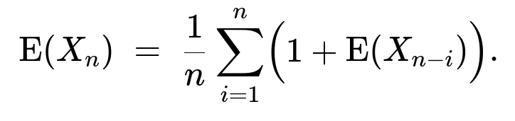
Here, (\text{E}(X_0) = 0) by definition, since with zero cars there are no clumps.
Solving the Recurrence
To see that the solution is the harmonic sum, one can expand the recurrence step by step. Alternatively, one can guess that (\text{E}(X_n) = H_n) where (H_n) denotes the (n)th harmonic number, (1 + 1/2 + 1/3 + \dots + 1/n). One checks that this guess indeed satisfies the recursion and initial conditions.
Thus, the closed-form expression for the expected number of clumps of cars is:

which grows approximately like (\ln(n)) for large (n).
Practical Example or Simulation
To give an intuitive sense of this result, one can simulate the scenario in Python:
import random
import statistics
import math

def simulate_clumps(n, num_simulations=10_000):
    # Speeds: random distinct values
    # We'll just assign random speeds, keep them distinct by sorting
    counts = []
    for _ in range(num_simulations):
        # Random ordering of 'cars'
        # In reality, each 'car' has a speed, but let's simulate by assigning random speeds
        speeds = [random.random() for _ in range(n)]  # random speeds
        # Pair each car with its random speed, then place them in some random order
        car_order = list(range(n))
        random.shuffle(car_order)
        # We track speeds in the same shuffled order
        ordered_speeds = [speeds[i] for i in car_order]

        clumps = 1
        current_min_speed = ordered_speeds[0]

        # Move from front to back and see if we form new clumps
        for i in range(1, n):
            if ordered_speeds[i] < current_min_speed:
                clumps += 1
                current_min_speed = ordered_speeds[i]
            else:
                # If it's faster, it has to slow down to current_min_speed
                pass
        counts.append(clumps)
    return statistics.mean(counts)

n = 10
sim_result = simulate_clumps(n)
theoretical = sum(1.0 / k for k in range(1, n+1))

print(f"Simulated average number of clumps for n={n}: {sim_result}")
print(f"Theoretical expected value (Harmonic number): {theoretical}")
Running such a simulation for various values of (n) will empirically show that the average number of clumps concentrates around the harmonic number (H_n).
Follow-Up Question 1
How does the result scale for large (n) and why?
Answer: For large (n), the (n)th harmonic number (1 + 1/2 + \dots + 1/n) grows asymptotically like the natural logarithm of (n). Concretely, (H_n \approx \ln(n) + \gamma), where (\gamma) is the Euler–Mascheroni constant ((\approx 0.5772)). Therefore, as (n) increases, the expected number of clumps grows approximately (\ln(n)). This is because each additional car has a decreasing probability of forming its own new clump, contributing successively smaller increments to the expected total.
Follow-Up Question 2
Could the distribution of speeds or positions affect the expected result?
Answer: No. The key is that we have (n) distinct speeds, all possible orderings of these speeds are equally likely, and the car positions on the highway (i.e., which car is first, second, etc.) are random. The exact continuous distribution from which the speeds are drawn does not matter as long as the speeds are almost surely distinct. What drives the result is the symmetry in placing these distinct speeds in a random permutation. Because each position is equally likely to host the slowest car (and similarly any ordered set of speeds is equally likely), the derivation holds for any continuous distribution of speeds.
Follow-Up Question 3
What if two or more cars could have exactly the same speed?
Answer: If ties in speed are allowed, the problem needs careful reinterpretation. In the original logic, we rely on having a single “slowest” car. If multiple cars share the same slowest speed, the clump analysis changes slightly because any of those slowest cars could form the “leading edge” of a clump. Nonetheless, if the probability of exact ties is negligible (which is typically the case with continuous distributions), the result remains the same. But for discrete or partially discrete distributions, we would need to account for the possibility of ties in the slowest speed. That can complicate the recursion but often does not drastically change the main result if ties are relatively rare.
Follow-Up Question 4
What if passing is allowed but at a cost or with some probabilistic rule?
Answer: Allowing cars to pass modifies the problem significantly because one of the main constraints that create clumps is removed or weakened. The mathematics behind expected clumps would need an entirely different setup, taking into account the probability of overtaking and the distribution of such events. In such scenarios, a car with a higher speed might overtake the slowest car and potentially avoid forming or merging into a clump. This would likely reduce the expected number of clumps, or at least alter how we must compute it. One would need to develop a new model, possibly incorporating Markov chains or continuous-time processes, to capture the transitions as passes occur.
Follow-Up Question 5
How does the recursion change if the slowest car could appear with a different probability (instead of uniform 1/n)?
Answer: In the standard problem, each car is equally likely to be the slowest because the speeds are distinct and drawn from a continuous distribution, making all orderings equally likely. If, however, we had a non-uniform “prior” on which car is slowest (for instance, if some cars are more likely to be slow due to mechanical limits), then the recursion would be weighted accordingly. Specifically, instead of summing over (i=1) to (n) with probability (1/n), we would have:
E(X_n) = sum over i=1..n [ p(i) (1 + E(X_{n-i})) ],
where p(i) is the probability that the slowest car is in position i. The recursion solution would then be tied to the exact form of p(i). The resulting expected value might no longer be a harmonic sum, but rather a weighted variant whose closed form would depend on the p(i) distribution.
Below are additional follow-up questions
How might the distribution of clump sizes be characterized beyond just the expectation?
When we calculate E(X_n), we only learn about the average number of clumps, not how those clumps might be sized or distributed. Analyzing the distribution of clump sizes can reveal, for instance, whether most clumps contain relatively few cars, or whether there's a significant chance of forming one huge clump that encompasses all cars.
To explore clump-size distribution, one approach is to consider how many cars are led by a particularly slow car. Each time we identify a new slowest car along the ordering from front to back, we can ask: "How many cars end up in this newly formed clump?" Studying those random cluster sizes often involves more complex conditional probability arguments. For example, in a small case with n=3 or n=4, one can list out all permutations of speeds and explicitly count the size of each resulting clump to derive distribution patterns. However, for larger n, a combinatorial explosion means we need more sophisticated methods or simulations to approximate the distribution.
From a practical standpoint, questions around how many clumps are small versus large can matter in scenarios such as traffic-flow analysis or supply-chain convoys, where knowing just the mean number of clumps might be insufficient.
What happens if each driver has a slight reaction time delay, causing potential gaps between cars that might break up clumps?
In the classic formulation, once a faster car encounters a slower car, it reduces its speed immediately and stays attached to that clump. However, real-world drivers do not change speeds instantaneously; there is a reaction time, and this could introduce spacing that might prevent cars from merging into a single jam under mild conditions. Sometimes, a faster driver might choose to maintain a slightly higher speed if the gap is large enough.
Modeling a reaction delay could mean that even if there is a “slowest” car, vehicles behind it might not strictly form one contiguous block. The presence of a time delay might permit occasional re-accelerations, or micro-passings, depending on how we incorporate rules for re-establishing speed. Hence, the expected clump count could increase slightly (because some cars that would have merged into one clump may form separate smaller clumps) or even decrease if delays cause them to slow down earlier and stay in a “rolling cluster.” The direction of the effect depends heavily on how we define the “clump formation” rule with these time delays.
Can external factors like road segments (e.g., traffic lights or toll booths) alter the recursion?
If the highway is segmented by external control points (traffic lights, toll booths, speed-limit changes), the independence and symmetry assumptions in our original problem might no longer hold. For example:
A traffic light could bunch up cars in front, resetting some of the speed order effects.
A toll booth might create forced merges or forced reorderings as some cars must slow more than others.
In any of these scenarios, the slowest-car-based symmetry breaks because cars’ positions and effective speeds after each checkpoint may no longer be a simple random permutation. Each checkpoint can reorder or separate cars unpredictably. Consequently, the simple recursion E(X_n) = 1/n * sum(...) might not apply as is. We would need a piecewise approach or a more complex dynamic model to capture how many clumps remain between these segments and how new clumps might form afterward.
How does the reasoning change if each car’s speed is not constant but follows some stochastic process?
When car speeds vary over time, the notion of “the slowest car” at one moment may not remain slowest later if speeds fluctuate. If we let each car’s speed be a random function of time (e.g., a Markov process), the formation of clumps is dynamic:
Two cars might be separated at one point in time but then converge into a clump if the lead car slows down or the trailing car speeds up to a point but still cannot pass.
A clump could even “split” if the leading vehicle accelerates above the trailing vehicle’s speed—although splitting might require an actual passing event, which is outside the original no-passing rule.
Hence, in truly time-varying settings (without the ability to pass), the concept of a permanent or “locked” clump might be replaced by transient states where cars group and ungroup at different times. Analyzing this would likely require continuous-time or discrete-time Markov models, and we could not rely on a single static ordering argument.
What if the highway has a finite length or the cars have to exit at a certain point?
In a finite highway scenario, especially if cars exit at different times, the formation and the duration of clumps can change substantially. For instance, a car near the end of the highway might exit before a trailing faster car can catch up to form a clump, thus reducing the total number of clumps observed at any snapshot in time. Conversely, a bottleneck at an exit ramp might increase the chance of clump formation.
When n cars travel a finite distance D, some may exit before merging with a slower group ahead, especially if the distance is not long enough for the speed differential to create overlap. This modifies the expected number of final clumps because the original model implicitly assumes an infinitely long road (enough distance for all merges to happen inevitably). In a finite-distance scenario, part of the challenge is calculating the probability that a car will catch up to the slower car in front within distance D.
What is the complexity of simulating large n, and could we use more efficient methods than direct simulation?
A direct simulation approach—where we generate random speeds, randomly permute them, and then iterate through the order to count clumps—has a complexity on the order of O(n) per simulation run. Doing many simulation runs might be computationally heavy for very large n. However, for the purpose of verifying a theoretical result like E(X_n) = H_n, a direct simulation is straightforward and still feasible for moderately large n (e.g., tens or hundreds of thousands of cars).
If we needed to simulate extremely large n, we could:
Use parallel processing to run multiple simulations concurrently.
Exploit that each simulation is dominated by sorting or random permutation generation (which is O(n log n) or O(n) for specialized methods).
Possibly use a known closed-form expression to reduce the need for large-scale simulation, confirming only small, medium, and a few large n values to check consistency with the theoretical formula.
Is there a straightforward way to interpret the result in terms of “record lows” in the sequence of speeds?
An alternative interpretation for the number of clumps is the count of “record minima” when reading speeds from front to back. Each time we see a speed that is strictly lower than all speeds encountered so far, we start a new clump. This viewpoint matches the slowest-car perspective in an incremental fashion: whenever a new slow speed appears as we go from the front of the line to the back, that new slowest speed leads a new cluster.
In fact, this problem is precisely the expected number of “record lows” in a random permutation. From this viewpoint:
Each position has a 1/k chance of being the new record minimum among the first k cars.
Summing up the probabilities 1/1 + 1/2 + ... + 1/n naturally yields the harmonic number.
This record-minima interpretation is often easier to understand. The pitfall is that one must confirm that “record minima in the order from front to back” truly aligns with clump formation under the no-passing rule. It does align here because each time we encounter a lower speed than all seen previously, that new speed will form a new “leading cause” of slowdown behind it, effectively starting a fresh clump.
How does this concept generalize to multi-lane highways with constraints on when or how cars can switch lanes?
In multi-lane highways, passing becomes feasible but may be restricted by traffic density or policy. Some complexities include:
If passing is allowed only with enough space in an adjacent lane, cars can “escape” from slow clumps, reducing the total number of clumps that form.
If multiple lanes exist but each lane has its own no-passing rule, we effectively treat each lane separately, but cars might change lanes randomly, introducing cross-lane interactions.
If the multi-lane highway merges back into a single lane, the merging segment can reintroduce the no-passing constraint, producing complex partial merges of clumps across lanes.
The biggest pitfall is to assume that the single-lane logic applies directly. Instead, multi-lane dynamics typically mean fewer, smaller, or shorter-lived clumps because cars have avenues to avoid being permanently stuck behind slower vehicles. Hence, the recursion involving the position of the slowest car does not directly translate. One might need a multi-dimensional state approach or a queueing-theory perspective to capture lane-switching behaviors.
What about modeling driver behavior or car preferences, such as some drivers always traveling slower when in close proximity to another vehicle?
In more realistic models, human factors can trump pure speed constraints. Some drivers may “brake-check” when they sense a car too close behind, causing faster cars to form clumps prematurely. Others may maintain a mandatory minimum following distance that affects exactly when merging into a clump occurs. These behavioral elements introduce random fluctuations that do not necessarily follow the simple distinct constant-speed assumption.
A pitfall is to over-rely on the neatness of the “slowest car splits the order” argument while ignoring real human driving patterns. In practice, any external or behavioral rule that changes how quickly a trailing car converges with the car in front can change the number of clumps. Nevertheless, for theoretical or idealized contexts (e.g., a line of robots or automated vehicles with no additional constraints), the original random-order argument remains perfectly valid.
In a queueing context, could we leverage Little’s law or other known results to validate or cross-check the harmonic number outcome?
Little’s law (L = λW) typically relates average number of items in a system (L) to the arrival rate (λ) and the average waiting time (W). While this problem is not exactly a queue in the typical sense—there is no well-defined arrival process or service discipline—it can still be interesting to consider if we can map it to a queueing scenario.
One possible mapping is to view each “clump” as a “server,” with the slowest car as a service-limiting factor for all cars that “arrive” behind it. However, this analogy often stretches the standard queueing assumption that jobs (cars) arrive independently rather than in a pre-arranged set of n. So while queueing theory might give some heuristics or partial insights, it does not trivially provide a direct alternative proof or consistency check unless carefully adapted.
The major pitfall here is that queueing systems typically assume an ongoing infinite or at least unbounded stream of arrivals, whereas we have a finite set of n cars that are randomly permuted. This difference limits how directly we can apply queueing equations.