ML Interview Q Series: Calculating Hidden Letter Probability in Drawers Using Bayesian Inference
Browse all the Probability Interview Questions here.
A desk has eight drawers. There is a 1/2 chance that a single letter was placed in exactly one of the eight drawers, and a 1/2 chance that no letter was placed in any drawer. After opening the first seven drawers and seeing that none contain a letter, what is the probability that the final drawer holds the letter?
Short Compact solution
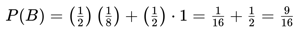
Let A represent the event that the 8th drawer contains a letter, and let B be the event that the first seven drawers are found empty. First, compute the probability of B by conditioning on whether a letter was placed at all. If a letter was placed, it is equally likely to be in any of the eight drawers, so the probability that it is not in the first seven drawers is 1/8. If no letter was placed, then obviously the first seven are empty. Thus:
Next, the probability of both A and B happening (i.e., the letter is specifically in the 8th drawer and the first seven are empty) is:

Finally, we use conditional probability:

Comprehensive Explanation
Bayesian Perspective and Intuition
The problem can be interpreted as a Bayesian inference scenario where we have two hypotheses:

Before checking any drawers, each hypothesis has a prior probability of 1/2. We then observe that seven of the drawers are empty:
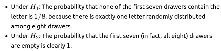
Hence, the observation “first seven drawers are empty” is more likely if no letter was placed, but it can still be consistent with there being a single letter in the 8th drawer.
We combine these likelihoods (the probability of seeing seven empty drawers given each hypothesis) with their respective priors. This yields:

Weighting by the prior (1/2 each), the total probability of seeing the first seven empty drawers is:

Then the conditional probability that the 8th drawer has the letter given the first seven are empty is

This aligns perfectly with our short derivation.
Why the Probability Is 1/9
A crucial point is that the event “seven drawers are empty” is heavily influenced by the possibility that no letter was placed at all, which increases the overall probability that all checked drawers turn out empty. Since that scenario (no letter placed) has an equal prior weight of 1/2, it strongly contributes to the observation that the first seven are empty. Hence, conditional on that observation, it’s not as likely that a letter was actually placed in the first place—leading to a relatively smaller fraction of the probability mass going toward the scenario where the 8th drawer actually contains the letter.
Bayesian Formula

So


Thus:

Hence

Alternative Perspective (Frequentist View)
Another way to see this is to imagine a large number of trials. In half of the trials, no letter is placed (and you always see all drawers empty). In the other half, one letter is placed in exactly one random drawer out of eight. Of those trials where you open 7 drawers and see no letter, you’d have:
Many trials from the “no letter placed” bucket (because it’s easy to see 7 empty drawers if no letter exists at all).
Fewer trials from the “letter is placed” bucket where the letter specifically lands in the 8th drawer.
Counting the ratio of these conditions leads to the 1/9 figure as well.
Potential Follow-Up Questions
How would you generalize this result to n drawers instead of 8?
When there are n drawers, the probability that a single letter is placed in exactly one drawer might still be 1/2, and the probability that no letter is placed is also 1/2. If you open (n−1) drawers and find them all empty, the same Bayesian argument applies. Specifically, if we label the event B = “first (n−1) drawers are empty,” and A = “the $n$th drawer has a letter,” we would do:
P(B) under the scenario of one letter (which has prior 1/2) is 1/n, because to find the first (n−1) empty means the letter is in the nth drawer.
P(B) under the scenario of no letter (which has prior 1/2) is 1, because all drawers are empty in that case anyway.
Hence:

The probability that the nth drawer contains the letter and the first (n−1) are empty is:

So


What if the probability of placing a letter was not 1/2 but some other value p?
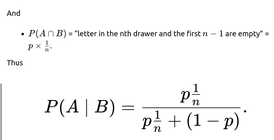
If p is the probability that exactly one letter is placed in one of n drawers, then (1−p) is the probability that no letter is placed. The logic is very similar:
P(B)= “first n−1 drawers empty” =

So

You can simplify or leave it in that form depending on the problem requirements.
Could there be more than one letter in the drawers?
This changes the assumptions drastically. If there could be multiple letters, the logic we used that “each drawer is equally likely to be the only one containing a letter” would no longer apply. We would have to define a new model for how many letters might be placed, and how they are distributed across drawers. The main principle of Bayesian inference would still hold, but the computation for P(B) (the event of first n−1 drawers being empty) and P(A∩B) (the event the $n$th drawer is non-empty and the rest are empty) would need to be recalculated accordingly. For example, if we assumed a Poisson or binomial distribution on the count of letters, the probabilities of seeing empty vs. non-empty drawers would differ significantly.

Could we run a simulation to confirm this probability?
Yes. A Python simulation can illustrate this result. For example:
import random

N = 10_000_000
count_event_B = 0  # count of times first 7 drawers empty
count_A_and_B = 0  # count of times 8th drawer has letter AND first 7 empty

for _ in range(N):
    # Step 1: Decide if a letter is placed
    # p_letter=0.5, so half the time place a letter in exactly one of 8 drawers,
    # otherwise no letter
    if random.random() < 0.5:
        # A letter is placed in exactly one random drawer
        letter_drawer = random.randint(1,8)  # 1 to 8
        # Check if the first 7 are empty
        if letter_drawer > 7:
            # Then the first 7 are definitely empty
            count_event_B += 1
            # Also check if 8th drawer is the letter
            if letter_drawer == 8:
                count_A_and_B += 1
        else:
            # The letter is in one of the first 7
            # so that means first 7 are not all empty
            pass
    else:
        # No letter
        # Then the first 7 are obviously empty
        count_event_B += 1
        # But there's no letter in the 8th
        # so no increment of count_A_and_B
        pass

# Probability of B = first 7 empty
p_B = count_event_B / N
# Probability of A and B = 8th has letter and first 7 are empty
p_A_and_B = count_A_and_B / N
# Probability of A given B
p_A_given_B = p_A_and_B / p_B
print("P(A|B) from simulation =", p_A_given_B)
Running this simulation should yield results close to 1/9≈0.111...
What if we discovered the letter distribution after partial knowledge?
In real-world scenarios, you might have partial knowledge, such as: “People are more likely to place letters in top drawers,” or “The chance of placing a letter is not exactly 1/2 but depends on the day.” Any partial information changes the prior distribution. The Bayesian update formula remains the same in structure, but you incorporate the new prior probabilities based on that partial knowledge. The numeric results would change accordingly.
These various follow-ups emphasize that once you clearly specify how letters are placed (the prior), how you gather data (i.e., checking drawers), and the likelihood function (the chance of seeing a certain pattern of empty vs. non-empty drawers given each hypothesis), you can apply Bayesian reasoning in a straightforward manner to compute the posterior probability.
Below are additional follow-up questions
What if the letter might have been removed or lost after being placed?
One potential complication is that the letter could have been placed initially, but then someone removed it from one or more drawers with some probability. This scenario changes the underlying assumptions about the probability that a given drawer contains a letter at the time of inspection.
Detailed Explanation
Initial Placement Model Suppose we retain the initial idea that there is a probability p (or 1/2 in the original problem) that the letter was placed in exactly one of n drawers. If it was placed, each drawer is equally likely to have received it.
Removal Model Now introduce a probability r that if a letter had been placed, it gets removed from its drawer before we check. In other words, even if a drawer was the one chosen for the letter, there is a chance r that we find it empty because the letter was taken away.
Observation Upon opening the first n−1 drawers, we observe they are empty. Under this new model, “empty” can arise either from the letter never having been placed in that drawer or from it being placed and subsequently removed.
Bayesian Update The probability of seeing n−1 empty drawers depends on:
The “no-letter” hypothesis (probability 1−p). Under this hypothesis, it is trivial that all n−1 drawers are empty.
The “letter-placed” hypothesis (probability pp. Given that the letter was placed in one specific drawer:
If the letter happens to be in one of the first n−1 drawers, we have to factor in the removal probability r (which would lead to emptiness upon inspection).
If the letter was placed in the $n$th drawer, then obviously the first n−1 are empty—no removal needed for those drawers. You would then need to carefully write down the probabilities reflecting these cases and solve for P(letter in nth drawer∣all first n-1 empty).
Edge Cases
If r=1, that means any letter placed is always removed; effectively, we never find any letter, so the probability that the $n$th drawer contains a letter at inspection time is zero.
If r=0, we revert to the original problem.

Does the order in which we check the drawers matter for the final probability?
A reasonable question is whether checking the first seven drawers in a specific sequence versus checking them in a random order would change the conditional probability that the last drawer holds the letter.
Detailed Explanation
Symmetry Argument In the basic setup where each drawer is equally likely to hold the single letter (if a letter exists), the probability of all seven checked drawers being empty does not depend on which physical drawers you opened first. It only matters that you have observed seven distinct drawers with no letter. Hence, the event “the first seven opened drawers are empty” has the same probability no matter the order or which drawers you pick to open.
Bayesian Perspective If there is no difference among drawers (i.e., uniform prior) and you have discovered emptiness in exactly seven distinct drawers, there is only one drawer left. The probability that it is non-empty depends purely on the prior chance that a letter was placed and not found in one of the other seven. Order of revelation doesn’t affect the final calculation under these assumptions.
When It Might Matter
If some drawers had a higher probability of containing the letter, then the order or choice of which drawers you check first does matter, because discovering emptiness in a “high-probability” drawer is more informative than discovering emptiness in a “low-probability” drawer.
If the act of opening a drawer can alter the state of the other drawers (e.g., some physical effect that might shift the letter), then the order would again matter, but that goes beyond the assumptions of the original scenario.
Thus, under uniform and independent assumptions, the probability remains the same. A pitfall is assuming that remains true if drawers are not equally likely or if checking them in a particular order changes your knowledge differently.
How might this logic extend if we can only partially inspect a drawer and aren't fully certain it's empty?
Sometimes, practical constraints mean you cannot conclusively determine emptiness. For example, each drawer might have a hidden compartment. You check quickly but there’s a certain chance you missed the letter.
Detailed Explanation
Modeling Uncertainty Let’s say each drawer you inspect has a probability q of being confirmed correctly. With probability (1−q), you might incorrectly deem it empty even if it actually contains the letter.
Implications for Observations Observing a drawer as “empty” doesn’t definitely mean it’s empty; it could be that you missed the letter. So your likelihood of observing “empty” must be adjusted:
If the drawer is truly empty, you see it empty with probability 1(assuming no false positives).
If the drawer does contain the letter, you still might see it empty with probability (1−q) because you might have overlooked it.
Bayesian Update The event B = “I observe all 7 drawers are empty” is now more likely than true emptiness alone might suggest, because of possible inspection error. The posterior probability that the letter is actually in the 8th drawer would require factoring in both:
The probability that the letter was never placed.
The probability that the letter was placed in one of the first 7 drawers but was missed.
The probability that it was in the 8th drawer (which we haven’t inspected yet) or that no letter exists.
Edge Cases
If q=1, we revert to the original scenario—no inspection error.
If q=0, all drawers appear empty no matter what; we gain no useful information. In that extreme case, checking any number of drawers does not update our belief at all.
The subtle pitfall is forgetting to account for the possibility of “observational miss.” This is particularly relevant in real-world tasks (e.g., mechanical compartments or electronic sensors that can fail to detect an object).
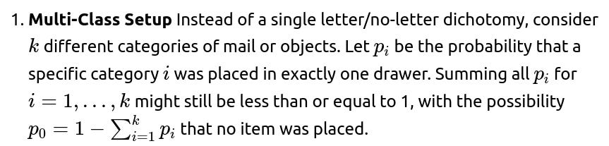
How would we handle multiple categories of objects (e.g., multiple types of letters) in the same set of drawers?
A real-world desk might contain not just one type of letter, but possibly different categories—some might have official documents, others might have personal letters, or none at all.
Detailed Explanation

2. Observation Model When you open a drawer, you check if it contains any item of interest. Seeing it empty rules out the presence of any one of those k categories, but does not differentiate which category might have been there if it were non-empty.
3. Bayesian Updating For each category i, we ask: “What is the probability that category i is in the 8th drawer given that the first 7 are empty?” This can be done using standard conditional probability, but now you sum across multiple categories:
The event “7 drawers empty” is more likely under “no letter at all” plus the sum of all possible ways one item of category i was placed in the 8th drawer.
The posterior for a specific category i being in the 8th drawer involves dividing the relevant joint probability by the total probability of seeing “7 drawers empty.”
4. Real-World Pitfalls
If categories have different likelihoods of being placed in the desk, that skews the posterior.
If some categories have a higher chance of being placed in multiple drawers, you need an even more detailed model.
Hence, we’d have a Bayesian approach for each category, and the final answer might be a distribution over categories: “The probability that the 8th drawer contains category 1 is X%, category 2 is Y%, or no letter is in there at all is Z%.”
Could the probability shift if we learn new information about the person who placed the letter or the day it was placed?
In practice, the assumption of a fixed probability of placing the letter (like 1/2) may be oversimplified if external context changes that probability.
Detailed Explanation
Adaptive Priors Let’s say historically, Person A places a letter 80% of the time they visit, while Person B places a letter only 20% of the time. If you discover that the person who visited the desk was Person A, your prior about “A letter is placed at all” should reflect that. Similarly, if the day of the week matters (e.g., a certain day is more likely to have mail), you might adjust the prior accordingly.
Observational Evidence If you know Person A is more organized and always places a letter in the top drawer if they do place one, that further modifies the distribution across drawers. Observing that the top drawer is empty is then a much stronger piece of evidence against the presence of a letter than if you had no such prior.
3. Implementation
Start with a prior p(letter) that depends on the person or the day.
Assign a distribution p(drawer∣letter placed) that might reflect usage preferences.
The event “empty in the first n−1 drawers” modifies your belief about whether the letter is present at all and, if so, where it is located.
Real-World Pitfalls
Overfitting: If you tune your priors too specifically based on limited anecdotal evidence, you might miscalculate.
Omitted variables: There could be other factors (e.g., is the desk locked? Is the letter urgent?) that also affect the probability of placement and the drawer chosen.
This highlights how real-world Bayesian reasoning often requires incorporating extra data (like personal habits) that shifts the prior probabilities well away from the simple 1/2 assumption.