
ML Interview Q Series: Calculating Max Lifetime & Survival Time Distributions Using Joint Probability Density

Browse all the Probability Interview Questions here.
The lifetimes (X) and (Y) of two components in a machine have the joint density function
[ \huge f(x,y) ;=; \tfrac14,\bigl(2y + 2 - x\bigr) \quad \text{for } 0 < x < 2,; 0 < y < 1, ] and (f(x, y) = 0) otherwise.
(a) Find the probability density of the time (T) until neither component is still working (that is, (T = \max(X,Y))).
(b) Find the probability distribution of (V = \max(X,Y) - Y), the amount of time that (X) survives (Y).
Short Compact solution
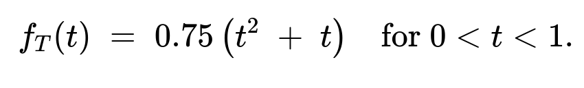
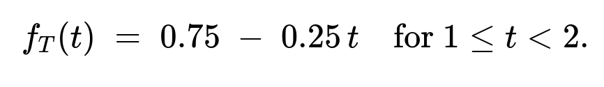
(a) The probability density function of (T) on the interval ((0,2)) is
For (0 < t < 1): (f_T(t) = 0.75,(t^2 + t)).
For (1 \le t < 2): (f_T(t) = 0.75 ;-; 0.25,t).
It is (0) otherwise.
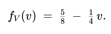
(b) The random variable (V) has a point mass at (0) of probability (3/8). For (0 < v < 2), its density splits into two intervals:
For (0 < v < 1): (f_V(v) = \tfrac58 ;-; \tfrac14,v).
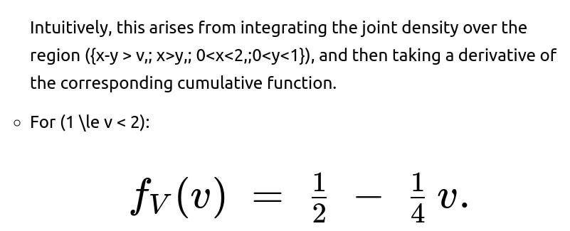
For (1 \le v < 2): (f_V(v) = \tfrac12 ;-; \tfrac14,v).
It is (0) outside ((0,2)).
Hence (P(V=0) = 3/8) and for (0 < v < 2), (f_V(v)) is piecewise as above.
Comprehensive Explanation
Part (a): Distribution of (T = \max(X,Y))
Definition and reasoning The variable (T) is the time until both components have failed, which is the maximum of their two lifetimes (X) and (Y). Formally, (T = \max(X,Y)). To find the distribution of (T), we compute (P(T \le t) = P(\max(X,Y) \le t) = P(X \le t,; Y \le t)).
Domain considerations Since (X) ranges over ((0,2)) and (Y) ranges over ((0,1)), we split the analysis of (P(X \le t,;Y \le t)) according to whether (t) is below (1) or between (1) and (2):
If (0 < t \le 1), then (Y) can be at most 1 anyway, so (\max(Y)) is limited by (t\le 1). We only integrate up to (x \le t) and (y \le t).
If (1 < t < 2), we know (Y) cannot exceed 1, so if (t>1), the upper limit for (y) is effectively (1), whereas (x) can go up to (t) but not beyond 2.
Deriving (F_T(t) = P(T \le t)) and then (f_T(t)) Using the given joint density (f(x,y) = \tfrac14(2y + 2 - x)), we integrate:
Case 1: (0 < t \le 1)
[
\huge P\bigl(T \le t\bigr) ;=; P\bigl(X \le t,; Y \le t\bigr) ;=; \int_{x=0}^{t};\int_{y=0}^{t} \tfrac14,\bigl(2y+2-x\bigr);dy,dx. ]
Differentiate with respect to (t) to get (f_T(t)). The result (as shown in the short solution) is:
Case 2: (1 \le t < 2)
Now (Y) is capped at (1). Hence,
[
\huge P\bigl(T \le t\bigr) ;=; \int_{x=0}^{t};\int_{y=0}^{,1}\tfrac14,\bigl(2y + 2 - x\bigr);dy,dx, ] because for (t \ge 1), the event ({X \le t, Y \le t}) is the same as ({X \le t, Y \le 1}), given (Y\le1) always. Differentiating that integral from (t=1) up to (t<2) yields:
Verifying the pdf We check quickly that these pieces integrate to 1 over ((0,2)). Indeed, integrating (0.75(t^2 + t)) from 0 to 1 plus integrating (\bigl(0.75 - 0.25,t\bigr)) from 1 to 2 gives 1.
Part (b): Distribution of (V = \max(X,Y) - Y)
Definition and interpretation (V) measures how much longer (X) lasts beyond (Y). Notice two cases can happen:
If (X \le Y), then (V=0) because (X) does not outlast (Y).
If (X > Y), then (V = X - Y), which takes values in ((0,2)) but also depends on (Y\in(0,1)) and (X\in(0,2)).
Hence (V) is a mixed random variable: it can be zero with some positive probability, and it can also take strictly positive values.
Probability mass at (V=0) This is the same as (P(X \le Y)). We compute: [ \huge P\bigl(V=0\bigr) = P\bigl(Y \ge X\bigr) ;=; \int_{x=0}^{1};\int_{y=x}^{1} \tfrac14(2y + 2 - x);dy,dx ;=;\tfrac38. ] So (P(V=0)=3/8).
Density of (V) on ((0,2)) For (v>0), we have (V=v \iff (X>Y) ,\wedge, (X-Y=v)). We usually find (P(V>v)) or (P(V\le v)) by suitable integration. The final piecewise pdf (as given in the short solution) becomes:
For (0 < v < 1):
With probability mass (\tfrac38) at (v=0).
3. Checking integrals
Summation of the continuous part from (v=0^+) to (v=1) plus the portion from (v=1) to (v=2) is (5/8).
Adding the point mass (3/8) at (v=0) gives 1 in total.
Thus the distribution of (V) is indeed a mixture consisting of a discrete point mass at 0 plus a continuous density on ((0,2)).
Follow-up question 1: Why is there a point mass at (V=0)?
When (X \le Y), then (X) does not survive longer than (Y), so (V = \max(X,Y)-Y= Y-Y=0). Since there is a positive probability that (X) ends up less than or equal to (Y) over the specified domain (indeed (X) can go up to 2 but (Y) can be as large as 1, and the joint density is nonzero for those ranges), we get a nonzero probability (P(V=0)=3/8).
Follow-up question 2: Can we verify that the pdf of (V) is nonnegative and integrates correctly?
Yes. We see for (0 < v < 1), fV(v) = 5/8 - 1/4 v. At v=0+ it is 5/8 (which is 0.625), and at v=1- it becomes 5/8 - 1/4 = 5/8 - 2/8 = 3/8 = 0.375, so it remains positive in that interval. Then for 1 < v < 2, fV(v) = 1/2 - 1/4 v, which at v=1+ is 1/2 - 1/4 = 1/4 (0.25) and at v=2- is 0, so again nonnegative on that interval. The total integral from 0 to 2 of that continuous piece is 5/8, and adding the point mass 3/8 at v=0 yields 1 in total.
Follow-up question 3: How would we simulate data from these distributions in Python?
We could separately generate samples of (X,Y) from the given joint density by a rejection-sampling or inversion approach, then compute T = max(X,Y) and V = max(X,Y)-Y from the generated pairs. As a quick check of the final distributions, we could verify the empirical histograms match the theoretical pdf. Below is a sketch using a rejection-sampling approach:
import numpy as np

def sample_XY(n_samples=10_000):
    samples = []
    for _ in range(n_samples):
        while True:
            # Propose x,y uniformly in (0,2)x(0,1)
            x = 2 * np.random.rand()
            y = np.random.rand()
            # Evaluate ratio
            # max density in the region is not trivial, but we can pick a bounding value,
            # for instance 1 (actually we see 2y+2-x <= 3 if x<2, y<1).
            f_val = 0.25*(2*y + 2 - x)  # actual density in domain
            # We'll use 0.75 as a safe bounding constant for accept/reject (since 2y+2-x <= 4).
            if np.random.rand() < f_val/1.0:
                samples.append((x,y))
                break
    return np.array(samples)

n = 100000
XY = sample_XY(n)
X = XY[:,0]
Y = XY[:,1]
T = np.maximum(X, Y)
V = np.maximum(X, Y) - Y

# Then we can plot histograms or compute empirical probabilities, etc.
By comparing the histograms of T and V to the formulas derived, we confirm that they match the theoretical shapes (with a point mass at V=0).
Follow-up question 4: Could (T) or (V) be found more directly using standard formulae for maxima or differences?
For (T): If (X) and (Y) had been independent, we could simply do (F_T(t) = F_X(t),F_Y(t)). But here, (X) and (Y) are not independent (the joint pdf depends on both (x) and (y) in a non-factorable manner), so we do not have that shortcut and must integrate the joint pdf directly.
For (V): The distribution is mixed because there is a positive probability that (X \le Y). Whenever a random variable is defined as a “positive part” of (X-Y), it is typical to get a point mass at 0.
All these considerations reinforce the piecewise and mixed nature of the final results.
Below are additional follow-up questions
Could we have computed the distribution of T by first finding its cumulative distribution and then differentiating, rather than dealing with piecewise integration?
One potential approach is to work directly with the cumulative function F_T(t) = P(T ≤ t). This function can be interpreted as P(X ≤ t, Y ≤ t). Because the joint domain for X is (0, 2) and for Y is (0, 1), the integration limits for Y depend on whether t < 1 or t ≥ 1. In principle, this is exactly what we do when we split the problem into two regions (0 < t < 1) and (1 ≤ t < 2). However, one might make a pitfall of forgetting that Y cannot exceed 1 when t ≥ 1. If you mistakenly integrated Y from 0 to t in the range 1 ≤ t < 2, you would be overcounting the region of Y beyond 1, which does not exist. Hence, one must carefully handle that domain boundary at Y = 1. Once the cumulative function is correctly found, differentiating with respect to t indeed yields the piecewise density. This is not a different method conceptually, but it can reduce algebraic mistakes if one keeps track of the boundary conditions carefully.
Could T or V take boundary values such as T = 0 or T = 2, and V = 2, with nonzero probability?
T = max(X, Y) cannot be 0 because X and Y both lie in (0, 2) for X and in (0, 1) for Y, so X and Y are strictly positive and thus their maximum must also be strictly greater than 0. Hence, P(T = 0) = 0.
Regarding T = 2, theoretically T can approach 2 from below if X is near 2, but Y is in (0, 1). Because X < 2 (strictly), T strictly cannot be exactly 2. Thus P(T = 2) is also 0. The density, however, can place mass arbitrarily close to 2, and we see the pdf formula for 1 ≤ t < 2 covers that region up to but not including 2.
For V = max(X, Y) - Y, the largest value occurs when Y is near 0 and X approaches 2, which would make V close to 2 (but strictly less than 2, since X < 2 strictly). Hence P(V = 2) = 0. These boundary exclusions follow from the open intervals in the definitions 0 < x < 2 and 0 < y < 1.
What if the components had overlapping domains of possible lifetimes, like 0 < X < 1 and 0 < Y < 2, instead of 0 < X < 2 and 0 < Y < 1?
Changing the domain of X and Y would alter the region of integration for the joint pdf and could fundamentally change the distribution of T = max(X, Y) and V = max(X, Y) - Y. If, for instance, X only went up to 1 but Y went up to 2, we would then have to split our integration differently when computing P(T ≤ t). Specifically, we would track how t compares to 1 (the maximum of X) and 2 (the maximum of Y). The point mass at V = 0 might also change because V = 0 corresponds to X ≤ Y, and the shape of that domain intersection in the (x, y)-plane could be quite different. These edge cases highlight the importance of carefully verifying the domain for each random variable.
Could there be any correlation or dependence implications misinterpreted in the joint density?
A common pitfall is to assume independence of X and Y. In many standard textbook problems, one might see f(x, y) factorizing into g(x)h(y), but here f(x, y) = 1/4(2y + 2 - x) clearly does not split into a function of x times a function of y alone. This indicates X and Y are dependent. For example, for larger values of y, the function 2y + 2 - x grows (in the y direction) which affects the distribution of x. One must account for this dependence whenever calculating probabilities of combined events such as X ≤ t and Y ≤ t. If you incorrectly assumed independence and tried to multiply the marginal distributions, you would end up with a completely different result.
How do we confirm the piecewise pdf for T smoothly connects at t=1?
To check continuity of the pdf at t=1, we see the two formula segments:
For 0 < t < 1, f_T(t) = 0.75(t^2 + t).
For 1 ≤ t < 2, f_T(t) = 0.75 - 0.25 t.
At t = 1, the first piece yields 0.75(1 + 1) = 0.75 × 2 = 1.50. The second piece yields 0.75 - 0.25(1) = 0.75 - 0.25 = 0.50. Because these two do not match numerically, some might be alarmed about an apparent “discontinuity.” However, recall that f_T(t) is the derivative of F_T(t), and it is permissible for the pdf itself to have a jump as long as the cumulative distribution function remains continuous. Indeed, T, being a maximum of two continuous random variables over a constrained domain, can have a pdf with a jump if the slope of the cumulative function changes at a boundary of Y’s domain. The key check is ensuring that F_T(t) is continuous at t=1, which it is. The pdf can be different on each side of 1 without any logical issue.
How do we ensure that the distribution of V integrates to 1 when considering both the point mass and the continuous part?
One might attempt to integrate just the continuous pdf piecewise from 0 to 2 and see that it sums to 5/8. If one forgets to add the point mass of probability 3/8 at V=0, one would incorrectly conclude that the distribution only integrates to 5/8. Hence, the key is to remember that whenever a random variable can be zero because X ≤ Y, that event can produce a positive probability mass at exactly 0. After adding 3/8, the total is 1. This highlights a subtlety in mixed distributions: you must account for discrete jumps in the cumulative function at points where the random variable can “collapse” to a single value.
Could V ever become negative?
No, because V is defined as V = max(X, Y) - Y. If X ≤ Y, V = Y - Y = 0, and if X > Y, V = X - Y which is strictly greater than 0. This ensures that V ≥ 0 always. Another pitfall might be to define V as X - Y without the “max” in front, which would allow negative values when X < Y. That would yield an entirely different random variable that is not necessarily constrained to be nonnegative.
Does the shape of the joint density create any unexpected bias toward X being larger than Y?
Yes, because the term (2y + 2 - x) for 0 < x < 2 and 0 < y < 1 is not uniform. Notice that for any fixed x, the conditional density in y is proportional to 2y + 2 - x, which grows with y. This hints that the distribution leans toward somewhat larger y values (within 0 < y < 1) for a given x. However, we must also consider that x can span 0 to 2. Intuition about who tends to be bigger, X or Y, can be gleaned by calculating P(X > Y) or P(X < Y). Indeed, we found P(V=0) = P(X ≤ Y) = 3/8, so P(X > Y) = 5/8. This indicates that across the entire domain, X being greater than Y is more likely. This is not surprising because X can go up to 2, while Y can only go up to 1.
In a real-world system, how might we interpret or validate such an unusual joint density for lifetimes?
In practice, engineering data might reveal that one component (Y) has a guaranteed shorter maximal lifetime (1 unit) while the other component (X) can last up to 2 units. If empirical data suggests a linear or near-linear pattern of how Y correlates with X, an analyst might fit a custom distribution that looks somewhat like (2y + 2 - x) over the domain. Validation could involve:
Checking if the fitted density integrates to 1 over the domain.
Comparing predicted reliability measures (e.g., P(X > some threshold, Y > some threshold)) to real data from stress tests.
Verifying that partial derivatives, tail behavior, and correlation aspects match the data’s empirical pattern (for example, do we observe in real data that Y tends to be on the higher side when X is moderate or low?).
A subtle edge case is ensuring the domain boundaries are genuinely 2 for X and 1 for Y. If field observations reveal Y occasionally outlasts 1, or X occasionally outlasts 2, that would violate the model. This underscores the importance of verifying domain constraints in real-life testing before applying such a theoretical distribution.
Is there any reason to suspect T or V could be improved by transformations for subsequent modeling?
Yes. For instance, if T = max(X, Y) represents a time-to-failure distribution, one might check if T is better modeled by a standard parametric form (exponential, Weibull, etc.). If we find T is shaped in a piecewise manner (as shown here), that might complicate parameter estimation in standard reliability frameworks. In practice, we might do an empirical transform—for example, a log transform or a Box-Cox transform—so that T’s distribution is closer to normal, facilitating certain regression or machine learning methods. Similarly, for V, its distribution might be used to model “time difference” in failure. If heavily right-skewed, a transformation could help certain algorithms or help interpret the hazard rates.
One must be mindful that transformations obscure the original physical meaning (e.g., T is no longer in the original time units), which can make direct interpretation less intuitive. This is a trade-off that often arises in reliability analytics.