ML Interview Q Series: Calculating E(X | X ≤ a) using Conditional Density: Exponential Distribution Example

Browse all the Probability Interview Questions here.

Let (X) be a continuous random variable with probability density function (f(x)). How would you define the conditional expected value of (X) given that (X \le a)? What is (E(X \mid X \le a)) when (X) is exponentially distributed with parameter (\lambda)?

Short Compact solution

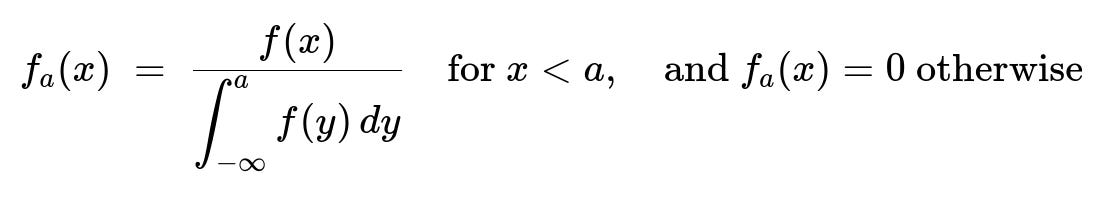
To define the conditional expectation (E(X \mid X \le a)), we first write down the conditional density of (X) given (X \le a). For (x<a), its conditional density is

Then, the conditional expectation is

When (X) follows an exponential distribution with rate (\lambda), that is (f(x)=\lambda e^{-\lambda x}) for (x\ge0) and (0) otherwise, one can compute

Comprehensive Explanation

Defining the conditional density

Suppose (X) is a continuous random variable with probability density (f(x)). We want to condition on the event ({X \le a}). By the definition of conditional probability for continuous distributions, the conditional density (f_a(x)) for (x < a) is:

• Numerator: the original density (f(x)).

• Denominator: the probability (\mathrm{P}(X \le a)), which is the integral (\int_{-\infty}^a f(y),dy).

Hence, for all (x<a),

f_a(x) = f(x) / ( ∫ from -∞ to a f(y) dy ), and f_a(x)=0 otherwise.

Conditional expectation

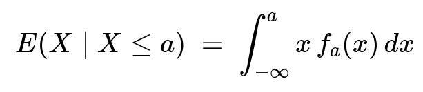
Once we have the conditional density (f_a(x)), the conditional expectation (E(X \mid X \le a)) is given by:

E(X|X ≤ a) = ∫ from -∞ to a [ x * f_a(x) ] dx.

Substituting (f_a(x)) in this integral:

E(X|X ≤ a) = ∫ from -∞ to a [ x * f(x) / ( ∫ from -∞ to a f(y) dy ) ] dx = (1 / ( ∫ from -∞ to a f(y) dy )) * ∫ from -∞ to a x f(x) dx.

Exponential distribution case

For an exponential distribution with rate (\lambda), the pdf is:

• (f(x) = \lambda e^{-\lambda x}) for x ≥ 0,

• (f(x) = 0) for x < 0.

To compute (E(X \mid X \le a)), we note that if (a < 0), then (\mathrm{P}(X \le a) = 0). Usually, we assume (a>0) so the condition ({X \le a}) is nonempty. Then:

1. Compute (\mathrm{P}(X \le a)) for a > 0: (\mathrm{P}(X \le a) = \int_0^a \lambda e^{-\lambda x},dx = 1 - e^{-\lambda a}.)

2. The conditional density of (X) for (x\in[0,a]) becomes: f_a(x) = [ (\lambda e^{-\lambda x}) ] / [1 - e^{-\lambda a} ].

3. Then,

E(X|X ≤ a) = ∫ from 0 to a [ x * f_a(x) ] dx = (1 / (1 - e^{-\lambda a})) * ∫ from 0 to a [ x * λ e^{-\lambda x} ] dx.

4. Evaluate the integral (\int_0^a x,\lambda e^{-\lambda x},dx). A straightforward way is integration by parts or using known definite integrals. The result is 1 - e^{-\lambda a} - \lambda a e^{-\lambda a} (after factoring out (\lambda) and performing the integration).

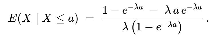
Putting these pieces together and dividing by (\lambda(1 - e^{-\lambda a})) leads to

E(X|X ≤ a) = [1 - e^{-\lambda a} - \lambda a e^{-\lambda a}] / [\lambda (1 - e^{-\lambda a})].

This quantity is strictly less than 1/λ (the unconditioned mean) because we are conditioning on being at or below a finite cutoff a. Intuitively, if the exponential random variable is forced to lie in the region [0, a], its average must be below the unconditional mean 1/λ.

Potential Follow-up Questions

1. What if (a < 0)? How do we interpret (E(X \mid X \le a)) for an exponential random variable?

If (a < 0) and (X) is exponentially distributed (supported on [0,∞)), then (\mathrm{P}(X \le a)) = 0 whenever a < 0. This means that the event (X \le a) is impossible. Thus the conditional expectation (E(X \mid X \le a)) is undefined (or does not make sense) for a < 0 in the case of an exponential distribution.

In a more general distribution with support extending into negative values, (\mathrm{P}(X \le a)) might be non-zero, and then you can compute the conditional expectation in the usual manner. But for an exponential random variable with parameter (\lambda), the probability is zero for any negative threshold.

2. Could you outline the integral steps for computing (E(X \mid X \le a)) in the exponential case?

Certainly. We want:

E(X|X ≤ a) = (1 / (1 - e^{-λa})) * ∫ from 0 to a [ x * λ e^{-λx} ] dx

Here is a brief outline:

1. Let I = ∫ from 0 to a [ x λ e^{-λx} ] dx.

2. Use integration by parts with u = x, dv = λ e^{-λx} dx. Then du = dx, and v = -e^{-λx}.

3. Evaluate at the boundaries 0 to a.

4. Carefully plug I back into the fraction and simplify.

The final expression is:

[1 - e^{-λa} - λ a e^{-λa}] / [λ (1 - e^{-λa})].

3. Is there an intuitive explanation for why (E(X \mid X \le a)) < (E(X)) for an exponential distribution when a > 0?

Yes. An exponential distribution has support on [0,∞), and its mean is 1/λ. When you condition on the event that the random draw is at most a (rather than allowing it to take any nonnegative value), you are restricting the variable to a smaller region. Because the exponential distribution is skewed to the right, forcing an upper cap at a > 0 but less than the typical scale 1/λ cuts off the large possible values in the tail that would normally increase the mean. Therefore, the conditional expectation must drop below the unconditional mean.

4. Can we apply a similar formula for other distributions beyond exponential?

Absolutely. The same idea applies to any continuous distribution. You simply replace f(x) by the pdf of your distribution and then carry out the integrals:

1. Compute the conditional density f_a(x) = f(x) / ∫ from -∞ to a f(y) dy, for x < a.

2. Compute E(X|X ≤ a) by integrating x f_a(x) from -∞ to a.

The main difference is that you typically have to handle the integrals or partial integrations specifically for each distribution. For some distributions (e.g., uniform, normal, gamma, etc.), you can find closed-form expressions; for others, you may need numerical integration.

5. How might we compute (E(X \mid X \le a)) in Python for a general distribution?

Below is a simple example using Python. Suppose we have a user-defined PDF f(x) and a function that computes the CDF or partial integrals. We can numerically integrate to find:

import numpy as np
from scipy.integrate import quad

def f_pdf(x, lambda_):
    # Exponential PDF if x >= 0, 0 otherwise
    return lambda_*np.exp(-lambda_*x) if x >= 0 else 0.0

def conditional_expectation(f, a, params=()):
    # denominator: P(X <= a)
    denom, _ = quad(lambda y: f(y, *params), -np.inf, a)
    # numerator: ∫ x f(x) dx from -∞ to a
    num, _   = quad(lambda x: x*f(x, *params), -np.inf, a)
    return num / denom

# Example usage for an exponential distribution with lambda = 2 and a=1.0
lam = 2.0
a_val = 1.0
res = conditional_expectation(f_pdf, a_val, (lam,))
print(f"E(X | X <= {a_val}) = {res}")

In practice, you adjust f_pdf for your chosen distribution. The principle remains the same: numerically integrate up to a to get the partial probability and the partial first moment, then divide.

Below are additional follow-up questions

How does the notion of truncated distributions relate to E(X | X ≤ a), and what boundary conditions should we consider?

The expectation E(X | X ≤ a) is precisely the mean of the lower-truncated distribution of X at a. In more general terms, if X has a pdf f(x), then the truncated distribution on (−∞, a] is simply the original pdf restricted to (−∞, a] and scaled by the cumulative distribution function evaluated at a. The boundary conditions to watch for include:

• The lower endpoint of the original support. For example, if X is nonnegative (like an exponential), and a is below 0, then P(X ≤ a) = 0, making E(X | X ≤ a) undefined. • If a is large enough to include most of the mass of the distribution (for instance, a → ∞), then the truncated distribution converges to the original distribution, and E(X | X ≤ a) converges to E(X).

In practical scenarios, one must ensure that the event {X ≤ a} has nonzero probability. Additionally, numerical integration for truncated distributions can become challenging if a is extremely large or extremely small relative to the distribution’s scale parameters.

Does the exponential distribution’s memoryless property play a role in conditioning on X ≤ a?

The exponential distribution is known for its memoryless property, which typically states that P(X > s + t | X > s) = P(X > t). This property directly applies to conditioning on “X > a,” not on “X ≤ a.” For “X ≤ a,” we are looking at the left-tail portion, effectively removing all observations that exceed a. That operation destroys the memoryless property because we are no longer dealing with the full future behavior beyond a certain point; instead, we are clipping off all values above a. Hence, E(X | X ≤ a) does not inherit the simplicity that the memoryless property brings when conditioning on events of the form {X > something}.

A subtlety arises in real-world data: if we assume the memoryless property but then condition on an upper bound, that upper bound changes the distribution in a way that can mislead an interpretation based solely on the memoryless aspect. One should remember that memorylessness applies to right-tail conditioning, not left-tail truncation.

What is the limit of E(X | X ≤ a) as a → ∞, and can it exceed the unconditional mean?

If a → ∞, then the event {X ≤ a} essentially becomes the entire support of X for large a. So, E(X | X ≤ a) → E(X). For an exponential random variable with rate λ, we know E(X) = 1/λ. Therefore, in the limit as a grows unbounded:

E(X | X ≤ a) → 1/λ.

This quantity can never exceed the unconditional mean once a is finite. Indeed, for the exponential distribution, any finite a truncation removes the heavier tail portion, thus lowering the mean relative to 1/λ. Only as a → ∞ do we regain the full right tail, at which point E(X | X ≤ a) converges back to 1/λ.

How would you approach estimating E(X | X ≤ a) if λ is unknown and you only have empirical data?

If you suspect X is exponentially distributed but do not know λ, you can take two main approaches:

Parametric approach. Estimate λ from data via maximum likelihood or method of moments using the full sample. Then plug the estimated λ-hat into the closed-form expression for E(X | X ≤ a). This is straightforward but relies on the correctness of the exponential assumption.

Nonparametric or direct empirical approach. Collect all observations xi in the sample that satisfy xi ≤ a, then compute their simple average as an estimate of E(X | X ≤ a). This approach does not require distributional assumptions. However, if the sample size of observations less than or equal to a is small, the estimate can have high variance.

Pitfalls include: • If a is chosen too small, you might have very few data points ≤ a, leading to noisy estimates. • If a is too large, the truncated set might not differ much from the entire dataset, and you could lose any real advantage of truncation. • If the true distribution is not exponential, forcing an exponential parametric model can lead to bias in your estimated conditional expectations.

How does the hazard function perspective help in understanding E(X | X ≤ a)?

The hazard function h(x) for a continuous random variable is typically defined for x in the support of X as: h(x) = f(x) / (1 - F(x)), where F(x) is the cumulative distribution function. This function represents the instantaneous rate of occurrence of the event at time x, given survival up to time x.

When we focus on E(X | X ≤ a), we are effectively ignoring all outcomes above a, so the resulting truncated distribution has its own hazard-like characterization on (−∞, a]. One might interpret how quickly the distribution “accumulates” probability mass up to a, but once you cut off beyond a, the hazard function concept is less directly applied in the same form. In reliability contexts, we often look at truncated distributions from the right side (e.g., X ≥ a), so E(X | X ≤ a) is somewhat less common in that setting. Nonetheless, the hazard rate can offer insights into how the distribution’s risk accumulates in the interval [0, a], clarifying why the expected truncated value might be lower or higher depending on the shape of f(x).

How can numerical stability or integration issues arise when computing E(X | X ≤ a)?

Potential numerical pitfalls:

• If a is extremely large for an exponential distribution, then e^(-λ a) might underflow to zero in floating-point arithmetic, causing potential inaccuracies when calculating 1 - e^(-λ a) or expressions like λ a e^(-λ a). • If a is very close to zero in a distribution that has significant mass near zero (like an exponential with small λ), partial integrals can be very small or very large, leading to possible floating-point overflow/underflow. • Using naive quadrature or integration routines without adaptive error control may give poor approximations, especially if the function is sharply peaked or has heavy tails cut off by a.

To mitigate these issues, one can use: • Log-transformations for terms like 1 - e^(-λ a) to avoid direct subtraction when these numbers are close to each other. • Higher-precision libraries if standard double precision is insufficient. • Specialized numerical integration methods (e.g., adaptive quadrature) that handle tail integrals carefully.

In practical data-driven applications, is it always meaningful to compute E(X | X ≤ a), or could censoring and missing data complicate the analysis?

In many real-world scenarios, you might have right-censored data (e.g., in survival analysis, some subjects remain “alive” beyond a certain observation window). In that case, you do not directly observe X for these right-censored instances, only that X exceeded the last observed time. This missing information complicates attempts to directly compute E(X | X ≤ a) from raw data because you do not have full knowledge of whether X was truly ≤ a or simply unobserved.

You would typically employ specialized survival analysis methods, such as the Kaplan–Meier estimator, or parametric survival models that handle censored data properly. These methods can accommodate partial knowledge of the data’s distribution and correct for bias that arises if one simply discards or misclassifies censored observations.

Censoring is a frequent pitfall if not handled explicitly. Failing to account for it can lead to an underestimation or overestimation of E(X | X ≤ a), depending on how you handle the censored cases relative to the threshold a).