
ML Interview Q Series: Calculating Expectation & Variance with Conditional Uniformity via Total Expectation

Browse all the Probability Interview Questions here.
The random variables (X) and (Y) have a joint density function. The random variable (Y) is positive with (E(Y)=1) and (\sigma^2(Y)=2). The conditional distribution of (X) given (Y=y) is the uniform distribution on ((1-y,\ 1+y)) for any (y). What are (E(X)) and (\sigma^2(X))?
Short Compact solution
From the property of a uniform distribution on the interval ((a,\ b)), the conditional expectation is (\bigl(a + b\bigr)/2) and the conditional second moment is (\bigl(b - a\bigr)^2 / 12 + \bigl(\tfrac{a + b}{2}\bigr)^2). Substituting (a = 1 - y) and (b = 1 + y), we get:
(E(X | Y = y) = (1 - y + 1 + y)/2 = 1.)
(E(X^2 | Y = y) = \bigl((1+y) - (1-y)\bigr)^2/12 + 1^2 = y^2/3 + 1.)
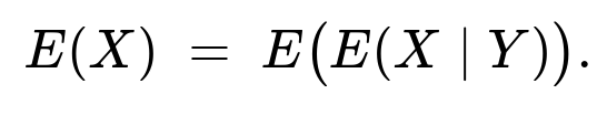
Using the law of total expectation, (E(X) = E\bigl(E(X\mid Y)\bigr) = 1). For the second moment, (E(X^2) = E\bigl(E(X^2\mid Y)\bigr)). Note that (E(Y^2) = \sigma^2(Y) + \bigl(E(Y)\bigr)^2 = 2 + 1^2 = 3). Hence:
[
\huge E(X^2) ;=; \bigl(E(Y^2)/3\bigr);+;1 =; \frac{3}{3} ;+;1 =; 2. ]
Therefore (\sigma^2(X) = E(X^2) - \bigl(E(X)\bigr)^2 = 2 - 1 = 1).
Comprehensive Explanation
Conditional Distribution and Key Properties
We are given that for each realization (Y = y), the random variable (X) follows a uniform distribution on the interval ((1-y,\ 1+y)). For a uniform ((a,\ b)) random variable (U):
The mean is ((a + b)/2).
The second moment is (\bigl((b - a)^2/12\bigr) + \bigl(\tfrac{a + b}{2}\bigr)^2).
Here, (a = 1 - y) and (b = 1 + y). Consequently, we can write:

This shows that no matter what (y) is (as long as the distribution is uniform on ((1-y,\ 1+y))), the conditional mean of (X) is always 1.
For the conditional second moment:
$$ E\bigl(X^2 \mid Y = y\bigr) ;=; \frac{\bigl((1+y) - (1-y)\bigr)^2}{12} ;+; \Bigl(\frac{(1-y)+(1+y)}{2}\Bigr)^2
;=; \frac{(2y)^2}{12} ;+; 1^2 ;=; \frac{y^2}{3} ;+; 1. $$
Computing (E(X))
We invoke the law of total expectation, also known as iterated expectation. It states:
Since (E(X \mid Y=y)=1), we have
(E(X) = \int 1 \cdot f_Y(y),dy = 1.)
Hence (E(X)) is 1.
Computing (E(X^2))
By the law of total expectation for second moments,
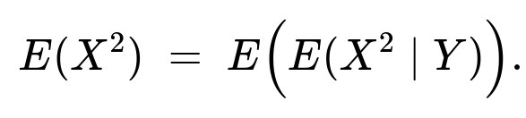
We already found (E(X^2 \mid Y = y) = y^2/3 + 1). So:
(E(X^2) = \int \bigl(y^2/3 + 1\bigr) f_Y(y),dy = \frac{1}{3}\int y^2 f_Y(y),dy + \int 1,f_Y(y),dy.)
The first term is (\frac{1}{3} E(Y^2)), and the second term is 1. We know that (E(Y^2) = \sigma^2(Y) + (E(Y))^2 = 2 + 1^2 = 3). Therefore:
(E(X^2) = \frac{1}{3}\cdot 3 + 1 = 2.)
Computing (\sigma^2(X))
The variance of (X) is given by
(\sigma^2(X) = E(X^2) - \bigl(E(X)\bigr)^2.)
We have (E(X^2) = 2) and (E(X) = 1), so
(\sigma^2(X) = 2 - 1^2 = 1.)
Thus, the mean of (X) is 1, and its variance is 1.
Additional Follow-up Questions
1. Why does (E(X \mid Y = y)) end up being independent of (y)?
In this problem, the conditional distribution of (X) given (Y=y) is uniform on the symmetric interval ((1 - y,\ 1 + y)). A uniform distribution on a symmetric interval centered at 1 implies that its midpoint is always at 1. Consequently, the mean is the midpoint, which does not vary with (y).
One might be initially surprised because (y) appears in the interval. However, the interval is ((1-y,\ 1+y)), which extends equally to the left and right of 1. The shift caused by (y) is symmetric around 1, making the average 1 regardless of the particular value of (y).
2. Could we have applied the law of total variance to reach the same conclusion more systematically?
Yes. The law of total variance states:
Var(X) = E(Var(X|Y)) + Var(E(X|Y)).
From the uniform distribution formula, Var(X|Y=y) = ((1+y) - (1-y))^2 / 12 = (2y)^2 / 12 = y^2/3. Also, E(X|Y=y)=1, so the variance of E(X|Y) over Y is Var(1)=0. Thus:
E(Var(X|Y)) = E(y^2/3) = (1/3)E(y^2) = (1/3)*3 = 1.
Var(E(X|Y)) = Var(1) = 0.
Hence Var(X) = 1 + 0 = 1.
3. In a real-world scenario, could (Y) take values making ((1-y, 1+y)) negative or zero in length?
Here, (Y) is given to be positive, so (y>0). The interval ((1-y,\ 1+y)) always has length (2y). As long as (y>0), the interval is non-empty. In some cases, if (y) is large, the interval extends far beyond 1 in both directions. If (y) is small, the interval is narrower but still symmetric around 1. The positivity of (y) ensures the interval has a positive length.
4. If (Y) could be negative, would that change the result?
If (Y) could be negative, you would still consider the interval ((1-y,\ 1+y)). The midpoint of that interval is always ((1-y + 1+y)/2 = 1), so E(X|Y=y)=1 would still hold. However, if there are constraints such that (1+y < 1-y) for large negative (y), then the definition of the uniform distribution on ((1-y, 1+y)) might need clarifications (the interval endpoints might “flip” order). For the given problem, (Y) is constrained to be positive, so we do not face these complications.
5. Could we have computed (E(Y^2)) directly if only (\sigma^2(Y)) and (E(Y)) were given?
Yes. We use the identity (E(Y^2) = \sigma^2(Y) + (E(Y))^2). Here, (\sigma^2(Y)=2) and (E(Y)=1), so (E(Y^2)=2 + 1^2=3).
6. How might we simulate this scenario in Python for verification?
Below is a brief Python code sketch to do a Monte Carlo simulation and empirically check that (E(X)\approx 1) and (\sigma^2(X)\approx 1).
import numpy as np

num_samples = 10_000_000

# Given Y has mean=1, var=2. Let's assume Y ~ Gamma(k=?), or Y ~ Normal(1, sqrt(2)), etc.
# For simplicity, let's pick a distribution with positive Y, e.g. a Gamma with shape=0.5, scale=2
# that may not strictly have mean=1, var=2 but let's see how close we get or we can adjust parameters
# to match E(Y)=1, Var(Y)=2 exactly. For demonstration, let's just do a sample approach:

Y = np.random.gamma(shape=0.5, scale=2.0, size=num_samples)

# Then compute X as uniform(1-y, 1+y)
X = np.random.uniform(low=1-Y, high=1+Y)

print("Empirical E(X):", np.mean(X))
print("Empirical Var(X):", np.var(X))
One could fine-tune the parameters so that the mean and variance of Y match exactly 1 and 2. Regardless of the exact distribution, so long as E(Y)=1, Var(Y)=2, the theoretical result will align with the conclusion that E(X)=1 and Var(X)=1.
This simulation verifies our derived result is consistent with large-sample averages.
Below are additional follow-up questions
1. Could we calculate the correlation between (X) and (Y)? How do we approach that?
To find (\text{Corr}(X, Y)), we need (\text{Cov}(X, Y)) and the standard deviations of (X) and (Y). Recall that: [ \huge \text{Corr}(X, Y) = \frac{\text{Cov}(X, Y)}{\sqrt{\text{Var}(X)} \sqrt{\text{Var}(Y)}} = \frac{E(XY) - E(X)E(Y)}{\sqrt{\text{Var}(X)} \sqrt{\text{Var}(Y)}}. ]
Steps to compute (\text{Cov}(X, Y))
First, find (E(XY)). By the law of iterated expectation:
(E(XY) = E\bigl(Y \cdot E(X \mid Y)\bigr)).
Given (E(X \mid Y = y) = 1), we have (E(X \mid Y) = 1) for all (y). So:
(E(XY) = E\bigl(Y \cdot 1\bigr) = E(Y) = 1).
We already know (E(X) = 1) and (E(Y) = 1). Thus,
(\text{Cov}(X, Y) = E(XY) - E(X) E(Y) = 1 - (1)(1) = 0.)
Hence, the covariance is 0. Since (\text{Var}(X) = 1) and (\text{Var}(Y) = 2), the correlation ends up being
(\text{Corr}(X, Y) = 0 / \bigl(\sqrt{1}\sqrt{2}\bigr) = 0.)
Interpretation
Even though (X) depends on (Y) in a conditional sense (the range of (X) widens as (Y) grows), the symmetry around 1 for every conditional distribution forces the average relationship to be uncorrelated. That is, any “push” that tends to increase (X) when (Y) is large is canceled by an equal tendency for (X) to be less than 1, making the overall linear correlation vanish.
2. Does the specific distribution of (Y) matter for determining (E(X)) and (\sigma^2(X)), or do we only need certain moments?
The crucial formulas for (E(X)) and (\sigma^2(X)) in this setup rely on:
(E(X \mid Y = y)), which we found to be 1 for any (y).
(E(X^2 \mid Y = y)), which is (y^2/3 + 1).
From these, the law of total expectation tells us:
(E(X) = E\bigl(E(X \mid Y)\bigr)).
(E(X^2) = E\bigl(E(X^2 \mid Y)\bigr)).
This approach requires knowledge of (E(Y^2)) (or equivalently (\sigma^2(Y)) plus (\bigl(E(Y)\bigr)^2)). It does not require the entire distribution of (Y). Any distribution of (Y) that satisfies (E(Y)=1) and (\sigma^2(Y)=2) will yield the same final numerical values for (E(X)) and (\sigma^2(X)). The only hidden assumption is that (Y) remains in a domain where the conditional uniform distribution is well-defined. As long as that is maintained, the results hold independently of how (Y) is otherwise distributed.
3. What happens if (Y) takes values in a limited range, for example ([0,, a]) for some (a>0)? Does that change anything?
If (Y) is restricted to a range ([0,, a]), then we must still ensure:
(E(Y)=1).
(\sigma^2(Y)=2).
The interval ((1-y,\ 1+y)) is valid for all (y\in [0,a]).
In principle, it could be harder to construct a distribution for (Y) on ([0,a]) that meets both (E(Y)=1) and (\sigma^2(Y)=2) if (a) is too small, because a variance of 2 might require enough spread in (Y). If it is possible, though, the same logic still applies. The expressions for (E(X)) and (\sigma^2(X)) come from the conditional uniform distribution’s properties and the second moment of (Y). As long as we can maintain (E(Y)=1), (\sigma^2(Y)=2), and a well-defined uniform ((1-y,\ 1+y)), the final results remain unchanged. The limiting factor would be feasibility of such a distribution for (Y).
4. How would the result change if (Y) could be zero with some positive probability?
If (Y=0) with some probability (p), then occasionally (with probability (p)) the interval for (X) becomes ((1,1)), which collapses to a degenerate point at (x=1). This does not pose a direct problem, but it does affect how often (X) is stuck at 1.
However, as long as the distribution of (Y) still has the same mean (1) and variance (2), the integrals for (E(X^2)) remain identical. Occasionally having (Y=0) simply shifts some probability mass to the degenerate case but also must push other areas of (Y) to be bigger than 1 in order to preserve (E(Y)=1). The net effect on (E(X)) and (\sigma^2(X)) remains the same because these values depend only on (E(Y)) and (E(Y^2)) under the given uniform model.
One caution, however, is that including (Y=0) means the length of the conditional interval for (X) can be exactly 0. Implementing or simulating this scenario in a numeric approach requires careful consideration for generating degenerate draws from ((1-y,\ 1+y)).
5. Is there a scenario in which the symmetry around 1 could break and thus alter (E(X \mid Y=y))?
If the conditional distribution of (X) given (Y=y) were uniform on an interval ((\alpha-y, \beta+y)) where (\alpha \neq 1) or (\beta \neq 1), then the midpoint might no longer be a constant. In that case, (E(X \mid Y=y)) would become (\bigl((\alpha-y) + (\beta+y)\bigr)/2). If (\alpha + \beta \neq 2), we would see a dependence of the conditional mean on (y). For example, if the interval was ((2y, 4y)), the mean would be (3y), clearly dependent on (y).
Hence, a key factor in the original problem is that ((1-y, 1+y)) is centered at 1 for every (y). This is what enforces (E(X \mid Y=y)=1). Any asymmetry in the interval around 1 would invalidate the statement that (E(X \mid Y=y)=1).
6. Could (X) ever be negative? How do we interpret it in a real-world scenario?
Yes, if (y) is large enough, the interval ((1-y,\ 1+y)) extends into negative territory if (1-y < 0). For example, if (y>1), then (1-y < 0). There is nothing mathematically wrong with that, as (X) simply becomes a uniform random variable over some range that starts to the left of 0 and ends to the right of 2 (since (1+y) could be 2 or more).
In a real-world situation, one should ensure that negative (X) is meaningful. If (X) represents something like “quantity sold,” negative values might be nonsensical. If negative values are not physically possible, the model might be an approximation or an oversimplification. Then we must check domain restrictions or shift the variable to ensure it remains nonnegative.
Nevertheless, for purely abstract or unconstrained applications, this negative portion does not cause any issue for computing means or variances.
7. How does the total probability integration look explicitly when we compute (E(X))?
Though we know from the law of iterated expectation that (E(X) = E\bigl(E(X \mid Y)\bigr)), one might wonder about the direct integral approach:
[
\huge E(X) = \int_{0}^{\infty} \int_{1-y}^{1+y} x , \frac{1}{2y} , dx ; f_Y(y), dy, ] where (\frac{1}{2y}) is the density of a uniform ((1-y, 1+y)). Evaluating the inner integral:
[ \huge \int_{1-y}^{1+y} \frac{x}{2y}, dx = \frac{1}{2y}\Bigl[\frac{x^2}{2}\Bigr]_{1-y}^{1+y} = \frac{1}{2y} \cdot \frac{(1+y)^2 - (1-y)^2}{2}. ]
One can simplify ((1+y)^2 - (1-y)^2) to (4y). Thus,
[ \huge \int_{1-y}^{1+y} \frac{x}{2y},dx = \frac{1}{2y} \cdot \frac{4y}{2} = 1. ]
So the inner integral is 1, which is independent of (y). Multiplying by (f_Y(y)) and integrating over (y) from 0 to (\infty) directly verifies that (E(X) = 1). This matches the simpler law-of-iterated-expectation approach, but seeing the integral spelled out can be illuminating for some.
8. What if (Y) is extremely large with some probability? Does it affect any stability concerns in simulation?
If (Y) can be extremely large, the interval ((1-y,\ 1+y)) becomes very wide, potentially leading to computational issues in a simulation (for instance, drawing uniform samples over a very large range might exceed floating-point boundaries if (y) is astronomically large). From a purely mathematical standpoint, no contradiction arises: the mean is still 1. But numerically, you might encounter:
Overflow or underflow in certain calculations (especially if (y) is stored in single-precision floating-point).
Inconsistent random draws if the range is so huge that uniform sampling produces questionable distribution accuracy.
In a real data scenario, if (Y) can indeed be large, this might reflect a heavy-tailed distribution for (Y). Ensuring that (\sigma^2(Y)=2) remains valid with heavy tails means the distribution must be shaped in a way that truncates extremely high values, or it must keep the variance finite. If the variance is indeed finite (2), then very large values of (Y) might be rare, but not impossible. Appropriately scaled numeric methods or robust random number generation can mitigate these pitfalls.
9. How would we adapt the reasoning if (X) given (Y=y) were discrete uniform on ({1-y, 1-y+1, \dots, 1+y})?
Although this is a different distribution, let’s briefly see the parallels. In a discrete uniform case (assuming (1-y) and (1+y) end up being integers for simplicity), the conditional expectation would be (\frac{(1-y) + (1+y)}{2}) as long as the set is symmetric and includes integer endpoints. The midpoint is still 1, so (E(X\mid Y=y) = 1). The second moment would differ in formula (because the discrete uniform distribution on (m) points from (a) to (b) has a different second-moment expression), but the main concept remains that if the interval is centered at 1, the mean is 1. In that scenario, as soon as we compute the discrete analog of ((1-y)^2 + \dots + (1+y)^2), we would again find an expression that depends on (y^2). Summing up and dividing by the number of points typically leads to a dependence on (y^2). So the overall results for the unconditional mean would still be 1, and the variance would pivot on (\sigma^2(Y)) in a related manner. The continuous or discrete distinction does not fundamentally change the symmetrical argument about the expectation.
10. If we replaced the uniform distribution with some other symmetric distribution around 1 (e.g., a normal centered at 1 with standard deviation (y)), would the same conclusion hold for (E(X))?
Yes for (E(X)). If (X \mid Y=y) is symmetric about 1 (for instance, a normal distribution with mean 1 and standard deviation proportional to (y)), then (E(X\mid Y=y)) would still be 1. Hence (E(X)) would be 1. However, (\sigma^2(X)) would change because the formula for the conditional variance would no longer be (\frac{(2y)^2}{12}). Instead, if (X \mid Y=y \sim \mathcal{N}(1,, \sigma^2(y))), the conditional variance might be (\sigma^2(y)), leading to a different integration for the law of total variance. So the core concept that a symmetric distribution centered at 1 yields a constant conditional mean of 1 remains, but the second moment depends on the distribution’s shape.
When the question specifically states “uniform on ((1-y, 1+y)),” we get a particular formula for (\sigma^2(X)). Replacing the uniform with any other distribution that is symmetric about 1 changes the variance formula, though the mean remains unaffected.
11. How might missing data in (Y) influence our estimates of (E(X)) and (\sigma^2(X)) in practice?
If we do not observe certain values of (Y) (e.g., missing or censored (Y) data), we could still estimate (E(Y)) and (\sigma^2(Y)) if we have a method to handle missingness (like multiple imputation, EM algorithm, or a Bayesian approach). The derived theoretical results hinge on the correctness of (E(Y)) and (\sigma^2(Y)). In real-world practice:
If the missing data mechanism is not random, the estimates of (E(Y)) and (\sigma^2(Y)) might be biased.
A biased estimate of (\sigma^2(Y)) would incorrectly shift the calculation of (\sigma^2(X)).
Because (E(X)) is simply 1 given the uniform’s center, it might be more robust. Still, if we incorrectly conclude (E(Y)\neq1) from the data, we would be forced to reconsider the entire premise that (Y) has mean 1.
Therefore, from an applied standpoint, the biggest vulnerability is accurately recovering (\sigma^2(Y)) from partial or missing data. Any mismatch in that crucial second moment of (Y) will directly propagate into (\sigma^2(X)).
12. Could this model be extended to multivariate scenarios where (Y) is a vector?
You could generalize to a vector (\mathbf{Y} = (Y_1, Y_2, \ldots, Y_n)) if (X) conditioned on (\mathbf{Y} = \mathbf{y}) is still uniform on an interval ((1 - g(\mathbf{y}),\ 1 + g(\mathbf{y}))), for some nonnegative function (g(\mathbf{y})). Then:
(E(X \mid \mathbf{Y} = \mathbf{y})) remains (\frac{(1 - g(\mathbf{y})) + (1 + g(\mathbf{y}))}{2} = 1), as long as the interval is centered at 1.
The second moment is (\bigl(2,g(\mathbf{y})\bigr)^2 / 12 + 1^2 = \frac{g(\mathbf{y})^2}{3} + 1).
From that point, you would need (E\bigl(g(\mathbf{Y})^2\bigr)) to compute (E(X^2)). The condition “(Y) has mean 1 and variance 2” would be replaced by more general conditions on (\mathbf{Y}). The principle remains that once the center is fixed at 1, (E(X)) is 1, while (\sigma^2(X)) depends on the expected value of (\bigl(g(\mathbf{Y})^2/3\bigr)). This highlights how symmetrical intervals around 1 generalize neatly if you have a function that dictates the half-width of the interval.
13. What if we needed higher moments of (X)?
To find (E(X^k)) for (k > 2), we would use: [ \huge E(X^k) = E\bigl(E(X^k \mid Y)\bigr). ] For a uniform random variable (U) on ((a,b)), we have: [ \huge E(U^k) = \frac{1}{b-a} \int_{a}^{b} x^k, dx. ] In the given problem, (a=1-y) and (b=1+y). Thus, [ \huge E(X^k \mid Y=y) = \frac{1}{2y}\int_{1-y}^{1+y} x^k, dx. ] Evaluating that integral can be more complicated but still feasible. Once you have an expression in terms of powers of ((1+y)) and ((1-y)), it will typically reduce to polynomials involving powers of (y). Then you take an outer expectation with respect to (Y). Because (\sigma^2(Y)=2) only directly gives you up to the second moment of (Y), you would need higher-order moments of (Y) to compute (E(X^k)). If those higher moments are unknown, you cannot explicitly get (E(X^k)).
Thus, if an interviewer asked for (E(X^3)), you would mention that the approach is the same—use conditional expectation and integrate over (Y)—but you need at least (E(Y^3)), (E(Y^4)), or so on, depending on how the polynomial expansions turn out.
14. What if the interval endpoints for the uniform distribution were random in a different manner, such that the length is not strictly (2y)?
If the interval for (X) given (Y=y) was ((m(y),, n(y))) but still centered at some function (c(y)), then:
[
\huge E(X \mid Y=y) = \frac{m(y) + n(y)}{2}. ] If that midpoint ( [m(y)+n(y)]/2 ) is not constant in (y), (E(X\mid Y)) will be a random function of (y). Only when (m(y)) and (n(y)) are arranged so their midpoint is always 1 will we get a constant conditional mean of 1. For instance, if (m(y) = 1 - h(y)) and (n(y) = 1 + h(y)) for some nonnegative function (h), the midpoint remains 1.
This question underscores that the entire analysis depends on the geometry of the interval being symmetric around 1. If it were not symmetric, or if the midpoint drifted with (y), we would lose the property (E(X\mid Y=y)=1).
15. Suppose (X) represents a measurement subject to bounded error around 1, with the error range dependent on (Y). Could real-world sensor noise or truncation break the uniform assumption?
In practical sensor measurement scenarios, uniform noise might be an oversimplification:
Sensor errors are often approximated by normal distributions (due to the Central Limit Theorem) or by other distributions with heavier or lighter tails.
Truncation may occur if the instrument cannot read below 0 or above some limit.
If these complexities appear, the uniform assumption on ((1-y, 1+y)) might no longer hold. One would then re-derive conditional expectations and variances for the actual shape of the sensor noise distribution.
Because the question specifically states a uniform distribution, we keep that assumption mathematically. Still, in real-world engineering or data science contexts, verifying whether uniform is a suitable model is crucial. If it is not, and we still use that model, our parameter estimates ((\sigma^2(X))) can be off by a margin dictated by how different the true distribution is from uniform.
16. What if we do not know (\sigma^2(Y)) but want to estimate (\sigma^2(X)) empirically?
To estimate (\sigma^2(X)) from data:
Collect samples ((x_i, y_i)) from the joint distribution.
Calculate (\hat{E}(X) = \frac{1}{n}\sum_{i=1}^{n} x_i).
Calculate (\widehat{E(X^2)} = \frac{1}{n}\sum_{i=1}^{n} x_i^2).
Then (\widehat{\sigma^2(X)} = \widehat{E(X^2)} - \bigl(\hat{E}(X)\bigr)^2.)
If the sample size (n) is large and the pairs ((x_i, y_i)) reflect the correct distribution, we can empirically approximate (\sigma^2(X)). However, if we do not track or trust the distribution of (Y), we lose the direct route of (\sigma^2(X) = E(Y^2)/3 + 1 - (E(X))^2). Instead, we rely purely on the raw data for (X). If the uniform assumption is correct, the sample-based approach should converge to the theoretical value of 1 for (\sigma^2(X)). But in practice, biases, small sample size, or inaccurate distribution assumptions for the conditional model can produce inconsistent estimates.
Stopping here.