
ML Interview Q Series: Calculating Incomplete Sample Probability with Inclusion-Exclusion & Poisson Approximation.
Browse all the Probability Interview Questions here.
A random number is repeatedly drawn from {1, 2, …, 10}. What is the probability that not all of the numbers 1, 2, …, 10 show up in 50 drawings?
Short Compact solution
By applying the inclusion-exclusion principle, let Ai be the event that the integer i does not appear in any of the 50 draws. The probability that at least one integer fails to appear (i.e., not all 10 integers are present) is:

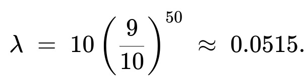
An approximate approach uses the idea that the number of distinct integers failing to appear follows a Poisson distribution with parameter
Hence the probability that at least one integer does not appear is

which is quite close to the exact result 0.0509.
Comprehensive Explanation
Inclusion-Exclusion Principle Approach
To determine the probability that not all of the numbers 1 through 10 appear in 50 independent draws from the uniform set {1, 2, …, 10}, one can define for each i in {1, 2, …, 10} an event Ai: “the number i does not show up in any of the 50 draws.” We then seek P(A1 ∪ A2 ∪ … ∪ A10).
According to the inclusion-exclusion principle, the probability of the union of these events is computed by alternately summing and subtracting the probabilities of intersections of these events. Concretely, we have:
The probability that a specific integer i never appears is (9/10)50, because in each draw the chance of picking something other than i is 9/10.
The probability that k specific integers do not appear is ((10-k)/10)50, because in each draw the chance of picking one of the remaining (10-k) numbers is (10-k)/10.
Hence the formula becomes a sum over k=1..10 of (−1)k+1 times the combinatorial factor for choosing which k integers fail to appear, multiplied by the probability that exactly those k integers all fail to appear. This yields:
(sum from k=1 to 10 of) [ (−1)k+1 * (10 choose k) * ((10 − k)/10)50 ]
Evaluating this sum numerically gives approximately 0.0509.
Poisson Approximation Intuition
An alternative viewpoint is to consider each of the 10 numbers independently and think about the probability that it is not drawn in 50 trials. For a single number, say number i, the chance that it does not appear at all is (9/10)50. Over 10 different numbers, define a random variable X = “the total count of integers from 1 to 10 that do not appear at all.” When 50 is fairly large relative to 10, X can be approximated by a Poisson distribution with parameter
λ = 10 * (9/10)50.
The event “not all 10 show up” is the event “X ≥ 1.” Thus, under the Poisson approximation:
P(X ≥ 1) = 1 − P(X = 0) = 1 − e−λ.
Numerically this is 1 − e−0.0515 ≈ 0.0502, which is close to the exact value 0.0509. The small difference comes from the fact that the Poisson approximation is only approximate—though it is typically quite accurate in such cases.
Why Both Methods Agree
The reason these two results are so close is that, for relatively large numbers of draws and a comparatively small set of possible outcomes (10 in this case), the number of missing integers follows a low-mean distribution. Poisson approximations often do well whenever the event of “missing a particular integer” has a small probability, and the events of missing different integers are not extremely correlated. Although there is some dependency (missing number 1 might slightly affect the probability of missing number 2), the approximation is still quite reasonable.
Interpretation in Practical Terms
In practical data sampling scenarios, this result means that after 50 uniform draws from 10 possible outcomes, there is around a 5% chance that at least one outcome is absent altogether. This is a relatively small but non-negligible probability. It indicates that if you want near certainty to see all 10 items at least once, 50 draws may not be quite sufficient for a guaranteed coverage (of course, you can never truly guarantee it with finite draws, but you can reduce the probability of missing items).
Potential Follow-Up Question 1
How would the formula change if we wanted the probability that all numbers 1 through 10 do appear at least once?
To find the probability that all 10 show up in 50 draws, we look at the complement of the event we just calculated. That probability is therefore:
1 − P(not all numbers show up).
In other words, 1 − 0.0509 = 0.9491 by the exact calculation. Using the Poisson approximation, it would be approximately 1 − 0.0502 = 0.9498. Thus the chance that every integer from 1 to 10 appears at least once in 50 draws is roughly 95%.
Potential Follow-Up Question 2
What if the draws are not equally likely for all 10 numbers? How would one approach that scenario?
If the draws are not uniformly distributed over {1, 2, …, 10}, then each integer i has some probability pi of being drawn on each trial, with the condition that the probabilities sum to 1. In that case:
The probability that number i does not appear in 50 draws becomes (1 − pi)50.
For the inclusion-exclusion principle, one would then consider for each subset of indices S in {1, 2, …, 10} the probability that all numbers in S fail to appear, which is ∏i in S(1 − pi)50.
We still alternate sums and differences in the same manner. The general formula would be:
(sum over all subsets S of {1,2,…,10} with S non-empty) of [ (−1)|S|+1 * ∏i in S(1 − pi)50 * (10 choose |S|) ]
but actually, we do not multiply by (10 choose |S|) in the same direct sense because each S is a distinct subset with its own probabilities. Instead, one enumerates each subset S, and the binomial factor only arises in the uniform case. In the non-uniform setting, we must precisely sum over all subsets of possible missing numbers, each with the appropriate product of (1 − pi)50, weighting by (−1)|S|+1. This approach is conceptually the same but more complicated to implement because there are 210 subsets to consider.
Potential Follow-Up Question 3
Why is the Poisson approximation valid, and under what conditions might it become unreliable?
The Poisson approximation comes from the idea that each integer “fails to appear” with a small probability, independently in many trials. More precisely, if the expected number of missing integers is λ (which is typically small for large numbers of draws), then the random count of missing integers tends to behave like a Poisson(λ) as 50 grows. This can break down if:
The probabilities pi differ significantly from each other (in the non-uniform case).
The correlation between events “missing i” and “missing j” is large (which can happen with a small number of draws or if one integer has a very high probability of appearing).
The sample size is not large enough so that the probability for a given integer not to appear is no longer “small.”
In those cases, the exact inclusion-exclusion or other approximations (such as the Chen-Stein method for Poisson approximation) might be needed to get an accurate estimate.
Potential Follow-Up Question 4
Could you illustrate how to implement a simulation in Python to estimate this probability?
Below is a straightforward Python approach that repeats the 50-draw process many times and records the frequency with which all 10 numbers appear at least once:
import random

def simulate_not_all_numbers(n_simulations=10_000_00):
    count_not_all = 0
    for _ in range(n_simulations):
        drawn_numbers = set()
        for _ in range(50):
            # Assuming uniform distribution from 1 to 10
            drawn_numbers.add(random.randint(1, 10))
        if len(drawn_numbers) < 10:
            count_not_all += 1
    return count_not_all / n_simulations

estimated_probability = simulate_not_all_numbers()
print("Estimated Probability (not all appear):", estimated_probability)
This code randomly generates 50 draws from {1, 2, …, 10}, checks how many unique numbers appeared, and tallies cases where some numbers are missing. Repeating for a large number of simulations n_simulations will give an empirical approximation of the probability. As n_simulations grows, the estimate converges (by the law of large numbers) to the true probability.
Such a simulation can be compared with the exact value 0.0509 (and the Poisson approximation 0.0502) to verify the accuracy of both approaches.
Below are additional follow-up questions
What happens if we only draw fewer than 10 times (e.g., 5 draws) and still ask about seeing all 10 numbers?
If the number of draws is strictly less than 10 (for example, 5 draws), it is logically impossible to see all 10 numbers. The probability that all 10 distinct numbers appear is then 0. Consequently, the probability that not all appear is 1. This edge case highlights that the formula using inclusion-exclusion will still give the correct probability of 1 (or extremely close to 1 if there was any approximation), but it’s a trivial situation from a combinatorial standpoint:
For k draws with k < 10, no matter how you pick the numbers, you can’t cover all 10 distinct possibilities.
This simple fact illustrates the importance of understanding domain constraints before applying any formula. If a formula is used blindly, you might forget that certain outcomes are outright impossible.
How do results change if the 50 draws are dependent rather than independent?
In many real-world scenarios, each draw might not be independent. For instance, if you have an urn with 10 labeled balls and you draw them one by one without replacement, the probability structure changes dramatically:
Without replacement: Once a number is drawn, its probability of appearing again is 0 in subsequent draws (because it’s physically removed from the urn).
Partial dependence: There might be correlation between consecutive draws in other ways, for example in a Markov chain setting.
When draws are not independent, the standard inclusion-exclusion approach for i.i.d. trials must be revisited because:
The probability of a number i not appearing across all draws is no longer simply (9/10)50.
You must carefully account for how each draw’s outcome updates the distribution for future draws.
Even though the logic of “defining events Ai” still holds, the intersection probabilities P(A1 ∩ A2 ∩ …) are different from the independent-draws assumption. One either has to derive a new combinatorial count for dependent draws or employ specialized tools (e.g., hypergeometric distributions in an urn-model scenario).
How would you generalize the formula to n total unique numbers and m draws?
The question about “not seeing all distinct outcomes” generalizes naturally if you have n possible outcomes and perform m draws (independently, with equal probability 1/n for each outcome). The event that not all n numbers appear in m draws is handled similarly by the inclusion-exclusion principle:
The probability that a specific subset S (of size k) of numbers does not appear is ((n − k)/n)m.
You sum over all nonempty subsets of {1, 2, …, n}, alternating signs according to (−1)|S|+1.
So the result is:
This becomes computationally more expensive for large n, since it requires summing up to n terms in the binomial expansion. For huge n, direct summation can be impractical and approximations (like Poisson or other bounding techniques) become more valuable.
How can we estimate the distribution (not just the probability) of the number of distinct integers obtained in 50 draws?
Sometimes, you want to know not merely the probability that all 10 appear but the full distribution over the number of distinct values seen. Let X be the random variable denoting “the number of distinct integers obtained in 50 draws.” You can compute P(X = k) for k=1..10 by:
Counting how many ways to choose exactly k distinct integers out of 10.
Ensuring each of the chosen k integers appears at least once.
Accounting for the fact that the total number of draws is 50.
More concretely:
Choose k distinct outcomes from 10: C(10, k).
Distribute 50 draws among these k chosen outcomes so that each chosen outcome appears at least once. This can be done using the number of ways to put 50 identical items into k distinct bins, each bin having at least 1 item (i.e., the number of integer solutions of x1 + … + xk = 50 with xi ≥ 1). That count is C(50−1, k−1).
Each allocation then has a probability (1/n)50 if the draws are all equally likely. But we also must consider permutations of the draws (since the draws themselves are ordered). One correct approach is the so-called “Multinomial coefficient” method. More advanced combinatorial arguments or direct usage of the occupancy problem are typically easier than a naive approach.
This distribution is often referred to as the occupancy distribution or coupon collector’s distribution. It’s more involved to compute explicitly for each value k, but it can be done either via exact combinatorial formulas or using computational routines. For large n or large m, the distribution also can be approximated using Poisson-based arguments or normal approximations, depending on the parameters.
How is the expected number of distinct integers in 50 draws computed, and why is it useful?
The expected value E[X] of the number of distinct integers X that appear in 50 draws (each equally likely among 10) is often simpler to calculate than the full distribution. We can use the linearity of expectation:
Let Ii be an indicator variable that is 1 if integer i appears at least once in the 50 draws, and 0 otherwise.
Then X = I1 + I2 + ... + I10.
E[X] = E[I1] + E[I2] + ... + E[I10].
But E[Ii] = P(Ii = 1) = 1 − P(integer i never appears) = 1 − (9/10)50.
Hence,

This quantity is useful because:
It tells you, on average, how many distinct numbers you see in 50 draws.
In the scenario with 50 draws and 10 equally likely outcomes, it also gives you a quick sense of coverage. For instance, if E[X] is around 9.5 or so, you’ll suspect that sometimes you do get all 10, sometimes you get 9 or fewer, and so on.
One pitfall here is that knowing E[X] alone does not give you the distribution or variance—so while the average might look reasonable, it might mask considerable variation. For example, it’s completely possible in some trials to see all 10, while in others you might see only 8 or 9 distinct values.