
ML Interview Q Series: Calculating Joint Car Buying Probability Using Set Theory and Complements.

Browse all the Probability Interview Questions here.
The probability that a visit to a particular car dealer results in neither buying a second-hand car nor a Japanese car is 0.55. Of those coming to the dealer, 0.25 buy a second-hand car and 0.30 buy a Japanese car. What is the probability that a visit leads to buying a second-hand Japanese car?
Short Compact solution
Let A be the event that a second-hand car is bought, and B be the event that a Japanese car is bought. We are given that P(A^c ∩ B^c) = 0.55, P(A) = 0.25, and P(B) = 0.30. We want to find P(A ∩ B).
Using the relationship that P(A ∪ B) = 1 - P(A^c ∩ B^c), we have:

Substituting the known values:
P(A ∩ B) = 0.25 + 0.30 - [1 - 0.55] = 0.25 + 0.30 - 0.45 = 0.10.
Therefore, the probability is 0.10 (i.e., 10%).
Comprehensive Explanation
Overview of Events and Complements
Define two events:
A: The event that the customer buys a second-hand car.
B: The event that the customer buys a Japanese car.
The complement of an event A (denoted A^c) is the event that A does not occur. So A^c means the customer does not buy a second-hand car, and similarly B^c means the customer does not buy a Japanese car.
Given data:
P(A) = 0.25. This means 25% of the dealer’s visits result in buying a second-hand car.
P(B) = 0.30. This means 30% of the dealer’s visits result in buying a Japanese car.
P(A^c ∩ B^c) = 0.55. This means 55% of the time, the customer buys neither a second-hand car nor a Japanese car.
We want P(A ∩ B), the probability that the customer buys a second-hand Japanese car.
Using the Formula for Unions and Complements
A key probability identity is:

It states that the probability of at least one of the events A or B occurring is 1 minus the probability that both do not occur.
We also know another fundamental set relationship:
Here:
P(A) is the probability of buying a second-hand car.
P(B) is the probability of buying a Japanese car.
P(A ∪ B) is the probability of buying either a second-hand car or a Japanese car (or both).
From the first formula, P(A ∪ B) = 1 - P(A^c ∩ B^c). We substitute that into the second formula:
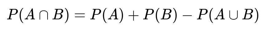
P(A ∩ B) = P(A) + P(B) - [1 - P(A^c ∩ B^c)].
Substituting the Known Values
We know P(A^c ∩ B^c) = 0.55, P(A) = 0.25, and P(B) = 0.30. Substituting:
P(A ∩ B) = 0.25 + 0.30 - [1 - 0.55] = 0.25 + 0.30 - 0.45 = 0.10.
Hence, the probability that a visit leads to buying a second-hand Japanese car is 0.10 (10%).
Why This Works
Intuitively:
25% buy second-hand (A).
30% buy Japanese (B).
55% neither buy second-hand nor Japanese (A^c ∩ B^c).
The complement of 55% is the 45% who buy “at least” one of the two types (A ∪ B). Among that 45%, some are second-hand only, some are Japanese only, and some are both second-hand and Japanese. We find the intersection by realizing that A ∩ B is included in each of the sums P(A) + P(B), but it is double-counted. Using the standard set formula accounts for this double counting.
Follow-up question: Could we visualize this with a Venn diagram?
Yes. In a Venn diagram approach:
The outer rectangle represents the entire sample space of all dealership visits (probability 1).
One circle represents the event A (second-hand cars).
Another circle represents the event B (Japanese cars).
The area outside both circles is A^c ∩ B^c, which is 0.55.
We know the total area of circle A is 0.25, the total area of circle B is 0.30, and the combined area of both circles is 1 - 0.55 = 0.45.
The overlapping region (A ∩ B) is what we want to find. By the typical Venn diagram formula, P(A) + P(B) minus the union area gives the intersection. That yields 0.10 for the overlap region.
Follow-up question: What if the events were mutually exclusive?
If the events A and B were mutually exclusive, their intersection (A ∩ B) would be zero. Then P(A^c ∩ B^c) would simplify differently. But in this problem, the events clearly are not mutually exclusive because it’s possible to buy a car that is both second-hand and Japanese. Indeed, the intersection is 0.10, which confirms that A and B do occur together in 10% of the visits.
Follow-up question: How to verify consistency of the given probabilities?
A good consistency check is:
P(A^c ∩ B^c) + P(A ∪ B) should equal 1.
P(A ∪ B) can be computed from P(A) + P(B) - P(A ∩ B).
We can confirm:
P(A^c ∩ B^c) = 0.55 P(A ∪ B) = 1 - 0.55 = 0.45
Then:
P(A) + P(B) = 0.25 + 0.30 = 0.55 P(A ∩ B) = 0.10
So P(A) + P(B) - P(A ∩ B) = 0.55 - 0.10 = 0.45, which is consistent with P(A ∪ B). Everything checks out.
Follow-up question: How might we extend this to more than two events?
When extending to three events A, B, and C, the union formula becomes more involved:
P(A ∪ B ∪ C) = P(A) + P(B) + P(C) - P(A ∩ B) - P(A ∩ C) - P(B ∩ C) + P(A ∩ B ∩ C).
The approach of using complements still works; for example, P((A ∪ B ∪ C)^c) = P(A^c ∩ B^c ∩ C^c). One has to account for all pairwise intersections and the triple intersection. In real-world problems, the logic is the same: we want to avoid undercounting or overcounting events when multiple overlaps exist.
Follow-up question: Could we simulate or check this with a quick Python snippet?
Yes. Although the problem is small enough to solve analytically, we can do a quick approximate check by simulating random Bernoulli draws. For instance:
import numpy as np

np.random.seed(0)  # For reproducibility
N = 10_000_000

# A occurs in 25% of cases
A = np.random.rand(N) < 0.25
# B occurs in 30% of cases
B = np.random.rand(N) < 0.30

# Force the portion of neither A nor B to 55%
# This is trickier in direct simulation because we must create correlation
# so let's illustrate a different approach: sample from categories.

# We'll produce an array of categories:
#  (A^c ∩ B^c) with 55%,
#  (A ∩ B^c) with X%,
#  (A^c ∩ B) with Y%,
#  (A ∩ B) with ?%
# so that the sums match 25% for A, 30% for B, 55% for none, 10% for both.

import random

categories = []
p_none = 0.55
p_second_hand_only = 0.25 - 0.10  # A only
p_japanese_only = 0.30 - 0.10     # B only
p_both = 0.10

for _ in range(N):
    r = random.random()
    if r < p_none:
        categories.append((False, False))
    elif r < p_none + p_second_hand_only:
        categories.append((True, False))
    elif r < p_none + p_second_hand_only + p_japanese_only:
        categories.append((False, True))
    else:
        categories.append((True, True))

A_sim = sum(1 for c in categories if c[0]) / N
B_sim = sum(1 for c in categories if c[1]) / N
A_and_B_sim = sum(1 for c in categories if c[0] and c[1]) / N
none_sim = sum(1 for c in categories if (not c[0] and not c[1])) / N

print("Simulated P(A):", A_sim)
print("Simulated P(B):", B_sim)
print("Simulated P(A and B):", A_and_B_sim)
print("Simulated P(neither):", none_sim)
This code crafts a distribution with exactly the probabilities we want. By construction, we’ll see approximately 25% for A, 30% for B, 10% for A ∩ B, and 55% for neither. This confirms the arithmetic we did is consistent.
All these details underscore how to handle basic set relationships and highlight the importance of avoiding double-counting in probability.
Below are additional follow-up questions
How can we verify that these given probabilities do not violate any fundamental probabilistic constraints?
One possible pitfall is to overlook whether P(A), P(B), and P(A^c ∩ B^c) are consistent in a fundamental sense. For instance, could P(A) + P(B) exceed 1 by a large amount that conflicts with the value of P(A^c ∩ B^c)? To verify consistency:
Check that 0 ≤ P(A^c ∩ B^c) ≤ 1. Here, 0.55 is valid because it falls between 0 and 1.
Check that P(A) + P(B) ≤ 1 + P(A ∩ B). Since we are told A and B are not necessarily exclusive, we ensure P(A) + P(B) = 0.25 + 0.30 = 0.55 does not exceed 1 + 0.10. Indeed, 0.55 ≤ 1.10.
Check that P(A ∩ B) ≥ 0 and P(A ∩ B) ≤ min(P(A), P(B)). We have 0.10 ≤ 0.25 and 0.10 ≤ 0.30, so that is also valid.
These checks confirm that the scenario is mathematically viable. In a real-world context, ensuring that measured probabilities for different events do not conflict in ways that break these basic bounds is often a key step before further modeling.
Are there any potential issues if we had erroneously assumed A and B were independent?
If we mistakenly assumed independence of A (buying a second-hand car) and B (buying a Japanese car), we would calculate P(A ∩ B) as P(A) * P(B) = 0.25 * 0.30 = 0.075. This is not equal to the actual intersection of 0.10.
Misapplying the independence assumption can lead to incorrect predictions about the number of customers who buy both second-hand and Japanese cars. In real-world scenarios, certain factors (e.g., cost considerations, brand preferences, supply constraints) might make these events positively or negatively correlated. Overlooking that correlation could lead to flawed business decisions, such as stocking too many or too few specific types of cars.
How would the problem change if we only knew conditional probabilities instead of absolute probabilities?
Sometimes, a question might provide something like P(A|B) or P(B|A) and ask for P(A ∩ B). For instance, if we knew P(A|B) = P(A ∩ B) / P(B), we could rearrange to get P(A ∩ B) = P(A|B) * P(B). Similarly, P(B|A) = P(A ∩ B) / P(A). We could combine such conditional probabilities with additional information about P(A), P(B), or P(A^c ∩ B^c) to deduce the missing intersection or union.
A pitfall arises if we only know partial conditional information without enough total probability data. For instance, knowing P(A|B) = 0.4 and P(B) = 0.3 alone is not enough to find P(A ∩ B) unless we assume the unconditional event is well-defined. Indeed, one must be sure that no contradictory information is lurking in the other probabilities.
Can we frame the problem as a Bayesian update scenario?
Yes, we could frame buying a second-hand car as prior knowledge about a customer’s purchase decision, then receiving new information (buying Japanese or not) could update the probability. For example:
We might initially have a prior P(A) = 0.25.
We learn the customer definitely bought a Japanese car (event B).
We then want P(A|B). Using Bayes’ rule in plain text: P(A|B) = P(A ∩ B) / P(B). In this scenario, we know P(A ∩ B) = 0.10 and P(B) = 0.30, so P(A|B) = 0.10 / 0.30 = 0.3333.
This means that if a person bought a Japanese car, there is a 33.33% chance it is also second-hand.
In a practical setting, auto dealers might refine marketing or inventory decisions based on these conditional probabilities (e.g., more marketing targeted to buyers who prefer Japanese cars if they also have a propensity to buy used).
Could the events be replaced with overlapping continuous variables instead of discrete events?
We can indeed think of “buying a second-hand car” and “buying a Japanese car” in a more continuous space—for example, a continuous random variable X denoting the age of the car, or a continuous random variable Y denoting some brand measure. In that scenario, we would define A as X > some threshold or B as Y in some category. The principle of complements and intersections remains the same. However, we would typically have integrals instead of sums:

where f_{X,Y}(x,y) is the joint probability density function. A pitfall is that we cannot simply do P(A) * P(B) to find P(A ∩ B) unless X and Y are independent. Real data may require sampling or integration based on the empirical joint distribution.
What if we only had frequentist counts from observed data rather than exact probabilities?
In many real-world dealership scenarios, we do not know the probabilities a priori. Instead, we collect data from N customers over a period. Let:
count(A) be the number of customers who bought a second-hand car.
count(B) be the number of customers who bought a Japanese car.
count(A^c ∩ B^c) be the number of customers who bought neither.
From these counts, we estimate:
P(A) = count(A) / N
P(B) = count(B) / N
P(A^c ∩ B^c) = count(A^c ∩ B^c) / N
Then we estimate P(A ∩ B) = P(A) + P(B) - [1 - P(A^c ∩ B^c)]. A common pitfall is sample size insufficiency or sampling bias. For instance, if the dealership only recorded partial data or did not track certain customers thoroughly, the computed probabilities might be skewed. Additionally, short observation windows might not capture true behavior if car buying is seasonal or cyclical.
Are there scenarios where these probabilities might evolve over time, and how would we handle that?
Yes, macroeconomic shifts, supply chain disruptions, or brand reputation changes can cause P(A), P(B), and P(A ∩ B) to fluctuate. For instance, a shortage of new cars might increase the probability that buyers end up with second-hand vehicles, or a new government policy might increase the appeal of certain Japanese models. We could model these as time-dependent probabilities P(A, t), P(B, t), etc. Then we might look at how P(A^c ∩ B^c, t) changes over intervals.
In practical terms, a pitfall arises if we assume stationarity (i.e., fixed probabilities) when in reality consumer behavior is dynamic. We would have to gather data over multiple time frames and either create a time series model or update our probability estimates incrementally to reflect new market conditions.
How do we handle the scenario if events A and B are not sharply defined?
Sometimes, “second-hand” might have nuances (e.g., certified pre-owned vs. used older than 10 years, etc.), and “Japanese” might also be fuzzy in real data collection (e.g., brand manufacturing location vs. corporate headquarters). If the event definitions are ambiguous, people collecting data might interpret them inconsistently:
Person 1 might classify a 6-month-old dealer demo car as second-hand.
Person 2 might classify only one-year-plus used cars as second-hand.
Similarly for “Japanese” cars: some might classify a brand name as Japanese even if the car is assembled in the U.S. The key pitfall is inconsistent labeling leading to internal contradictions in P(A^c ∩ B^c). The solution is to specify clear operational definitions for events.
If you do not standardize how A and B are defined, your measured probabilities can become unreliable or contradictory.
How important is it to check real-world correlations with domain expertise?
Sometimes a raw probability approach might overlook domain-specific causal relationships, like marketing campaigns that specifically target second-hand Japanese cars, or consumer preferences that might lead to strong correlation. For example, a new brand phenomenon might drastically increase the intersection P(A ∩ B) if used car dealers focus on certain popular Japanese models. If domain experts know such factors drive demand for certain combinations, they can guide adjustments to the basic formula or re-interpret the probability results.
A pitfall is ignoring domain insights and blindly applying set formulas without considering external influences. This might yield correct mathematics but poor real-world accuracy.
Could overlap among more categories complicate the analysis?
Yes. If we have more categories than just “second-hand” vs. “new” and “Japanese” vs. “non-Japanese” (for example, electric vs. gas, or domestic vs. imported from multiple regions), we must be careful in defining each event and possible intersection. For N categories, the event space can expand combinatorially, and we might need to apply the principle of inclusion-exclusion more extensively. The risk is double-counting or missing certain event overlaps.
In real-world analytics, applying the principle of inclusion-exclusion incorrectly can lead to large errors in inventory forecasts or marketing expenditures if we overestimate or underestimate the intersection of events.