
ML Interview Q Series: Calculating the Expected Minimum of Uniform Variables Using Probability Distribution Functions.

Browse all the Probability Interview Questions here.
Suppose X and Y are each independently drawn from a Uniform(0, 1) distribution. What is the expected value of their minimum?
Short Compact solution
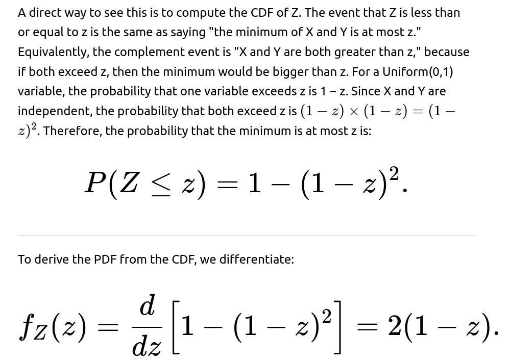
Let Z be the minimum of X and Y. Because both are i.i.d. Uniform(0,1), the cumulative distribution function for Z can be found by noting that:

Taking a derivative of this CDF with respect to z gives the probability density function of Z:

for 0 ≤ z ≤ 1. The expected value of Z follows from integrating z times this density from 0 to 1:

Hence the expected value of the minimum is 1/3.
Comprehensive Explanation
When X and Y are drawn uniformly and independently over the interval (0,1), each value within that interval is equally likely for both X and Y. The minimum of these two random variables, which we denote Z, will itself be a random variable that skews toward values close to 0.

Carrying out this integral yields:

That final result, 1/3, makes intuitive sense. Because the minimum of two uniform(0,1) variables tends to be smaller than the average of either one taken alone (which would each have expectation 1/2), we end up with a lower expected value. In fact, more generally, if you have n i.i.d. Uniform(0,1) random variables, the expected minimum is 1/(n+1).
Another way to verify this result is by performing a simulation. You can generate large samples of X and Y from Uniform(0,1), compute the empirical mean of the minimum, and you will see that it approaches 1/3 as the number of samples grows.
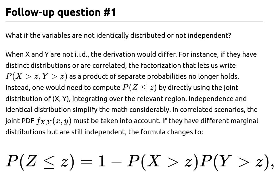
with each probability term depending on its respective distribution. In that case, to find E[Z], you would need to derive the PDF from that CDF in a similar manner. The final expression for expectation would no longer be 1/3, but would be an integral that involves the PDFs or CDFs of X and Y separately.
Follow-up question #2
What if we wanted the expected minimum of more than two i.i.d. Uniform(0,1) variables?

Using the same logic, we compute:

This result shows how the expected minimum becomes smaller as more uniform variables are included, which aligns with intuition.
Follow-up question #3
Can we verify the result using a double-integral approach?
Yes, there is an alternative method to compute E[min(X,Y)] by using a direct double integral. The minimum of X and Y can be expressed as:


Follow-up question #4
Can we quickly illustrate this result through a Python simulation?
Yes. Below is a simple Python script that uses NumPy to simulate a large number of samples for X and Y from Uniform(0,1) and then computes the sample average of their minimum. As the sample size grows, it should approach 1/3.
import numpy as np

np.random.seed(42)  # For reproducibility
n_samples = 10_000_000
X = np.random.rand(n_samples)
Y = np.random.rand(n_samples)

Z = np.minimum(X, Y)
estimate = Z.mean()

print("Estimated E[min(X,Y)] =", estimate)
When you run this code, you should see the output converge to approximately 0.333..., confirming the theoretical result of 1/3.
Below are additional follow-up questions
Follow-up question #1
How would one compute the variance of the minimum of X and Y, and why might the variance be useful in practice?
Answer: To compute the variance of the minimum, we need two ingredients: the first is the expected value of the minimum (which we already know is 1/3 for two i.i.d. Uniform(0,1) variables), and the second is the expected value of the square of the minimum. The variance can be expressed as
[ \huge \mathrm{Var}[\min(X,Y)] = E[\min(X,Y)^2] - \bigl(E[\min(X,Y)]\bigr)^2. ]
We find (E[\min(X,Y)^2]) by integrating (z^2) against the PDF of the minimum. Once we have that integral, we subtract the square of (1/3). In practical applications, the variance is valuable because it quantifies how spread out or volatile the minimum can be from one sample to another. If we’re doing a risk analysis or want to understand the worst-case performance metric where the minimum is relevant (for example, the lowest signal strength in a communication system or the smallest payoff in a game), having both the mean and variance of the minimum can guide decisions. For instance, even if the expected minimum is 1/3, a high variance might mean frequent occurrences of extremely small minimum values, influencing how we handle resource allocation, buffering, or error margins.
A subtle pitfall arises if we attempt to approximate the variance using too small a sample size. The minimum of a distribution is quite sensitive to outliers, so careful statistical techniques and sufficient sample size are necessary to get a stable estimate of its variance.
Follow-up question #2
What happens if we only observe (X, Y) within a restricted sub-range, say we only keep samples where both X and Y exceed 0.2? How does that affect the expected minimum?
Answer: Restricting the observed data to a sub-range can drastically alter the distribution of the minimum. When you throw away all samples where either X or Y is less than 0.2, you effectively create a truncated dataset. This truncation introduces bias into any direct calculation of the expected minimum, because the removed portion of the distribution (in which the minimum is below 0.2) is precisely where small values of the minimum occur. Thus, the computed mean of the minimum in this truncated sample will be larger than the true mean from the full (0,1) range.
To address such a scenario, one might have to account for the truncation by applying methods that re-weight or model the missing portions appropriately. If the reason for truncation is a measurement limitation (e.g., sensors cannot detect values below 0.2), a careful statistical correction method needs to be employed. Otherwise, any direct empirical average from the truncated range will systematically overestimate the true expected minimum.
Pitfalls here include:
Failing to account for the discarded portion of data leads to incorrect expectations.
If truncation is not random (e.g., you only record data within a certain region due to a sensor threshold), it introduces selection bias that must be modeled or corrected.
Follow-up question #3
What if we only have partially observed data? For instance, sometimes we see X but not Y, or vice versa. Can we still estimate E[min(X, Y)] accurately?
Answer: Partial observations and missing data complicate the estimation significantly. If values for one variable are missing at random and the other variable is fully observed, you cannot simply take the empirical average of the observed minimums because many minimum values may remain unobserved when the missing variable might have been smaller. Standard strategies include:
Imputation: You estimate the missing values of X or Y using statistical models, then compute the minimum on these completed data. However, imputation must be done carefully to avoid bias. If the missingness depends on the size of the variable (not missing at random), naive imputation can distort the distribution.
Likelihood-based Methods: In some advanced statistical frameworks, one can write down the joint likelihood for (X, Y) with partially missing data and then use maximum likelihood estimation or Bayesian methods to infer the distribution of the minimum.
Bounding Approaches: Sometimes you can derive upper and lower bounds for the expected minimum based on partial information about missing entries, especially if you have constraints on what values the missing variable could take.
A subtle pitfall is ignoring the dependency structure between the presence or absence of data and the actual value of the variable. If data is more likely to be missing when the value is small or large, that will induce biases that require specialized missing-data methods to correct.
Follow-up question #4
In a real-world scenario, the distribution might not be exactly Uniform(0,1). How would you test whether the assumption of uniformity is valid before applying the formula for E[min(X,Y)]?
Answer: One approach is to gather sample data for X and Y and use statistical tests or visual diagnostics to see if they resemble Uniform(0,1). For instance:
Q–Q Plots (Quantile–Quantile Plots): Plot sample quantiles against theoretical quantiles for a Uniform(0,1) distribution. If the points fall close to the diagonal line, that supports the uniform assumption.
Kolmogorov–Smirnov Test (K–S Test): This nonparametric test checks whether a sample comes from a given distribution. If the p-value is low, that suggests the data is not uniform.
Chi-Square Goodness-of-Fit: If you bin the data in sub-intervals of (0,1), you can compare observed frequencies with those expected under a uniform assumption.
If the distribution is found not to be uniform, applying the formula that yields 1/3 for the minimum would be invalid. Instead, you would need to re-derive the distribution of the minimum using the correct marginal distributions and any correlation structure, or at least adjust your approach to the actual distribution. A subtle real-world pitfall is that small deviations from uniformity in a tail region can significantly change the behavior of the minimum if that tail region is where extreme values occur.
Follow-up question #5
If we want to approximate the expected minimum in practice using a finite sample, what sample size considerations are relevant, and how can large deviations occur?
Answer: When empirically estimating the expected minimum from a sample of size N:
Sampling Error: Since the minimum can be heavily influenced by rare extreme values, one must consider whether the sample is large enough to capture the true distribution in the lower tail. Smaller samples might not encounter many extreme values, leading to an overestimate of the minimum.
Law of Large Numbers: Although the sample average converges to the true mean in theory, the speed of this convergence can be slow for tail-sensitive functions, like the minimum. You often need more samples to stabilize the estimate of E[min(X,Y)] compared to, say, E[(X+Y)/2].
Variance and Confidence Intervals: You typically want to construct confidence intervals around the sample mean of the minimum. Given the variance of the minimum can be relatively large compared to the variance of a more central statistic, more samples may be required to get tight confidence bounds.
A real-world pitfall is overlooking how quickly the sample minimum (even across pairs) can fluctuate from batch to batch. Additionally, if you gather data in batches or from different populations, changes in the underlying distribution can cause further deviations in your estimate.
Follow-up question #6
What happens if we apply a monotonic transformation to X and Y, such as taking the logarithm or squaring them, before computing the minimum?
Answer: A strictly monotonic transformation preserves the ordering of values but changes the distribution shape. For instance, if you transform X to log(X) and Y to log(Y), the minimum of these transformed variables does not correspond simply to the log of the original minimum. Instead, you are now dealing with a different random variable altogether. If your objective genuinely depends on the minimum of X and Y in the original scale, applying a transformation first would yield a statistic that might be less interpretable.
A subtlety is that sometimes transformations are performed for convenience or normalizing reasons. However, the expected minimum in the transformed domain might not reflect the original question of "what is the expected minimum in the original domain?" If the problem specifically needs the minimum in the original scale, you must either avoid the transformation or carefully transform back at the end (though the minimum of the log is not simply the log of the minimum, so you can’t just invert that final result in a straightforward way).
Follow-up question #7
How do we handle a scenario where X and Y can be negative, for instance if they’re Uniform(-1, 1), and we’re asked for the expected minimum?
Answer: When the domain extends into negative territory, the procedure is conceptually the same: find the CDF of the minimum and then integrate to get the mean. For example, if X and Y are i.i.d. Uniform(-1,1), you compute (P(Z > z) = (1 - F_X(z)),(1 - F_Y(z))), where (F_X) and (F_Y) are the CDFs of each variable. For Uniform(-1,1), the CDF is different from that of Uniform(0,1), so the corresponding expressions will yield a different result.
Real-world issues often arise because negative values can have special meanings, such as negative profits or losses in finance. It becomes important to interpret the distribution carefully. Negative domains can have corners or boundaries (like real-world constraints that values cannot drop below some limit), which might lead to piecewise distribution definitions. Any mismatch between the theoretical range and the actual feasible range of the variables can cause errors in the estimates.
Follow-up question #8
In a large-scale, distributed data collection setup (e.g., sensor networks), how might one efficiently compute or track the expected minimum of pairs (X, Y) without gathering all data in one location?
Answer: When data is distributed across multiple nodes, computing the minimum for each pair can be impractical if all data must be transferred to a central server. Some considerations:
Streaming or Online Algorithms: If X and Y arrive in real-time as streams, you can maintain partial statistics such as count, partial sums, and partial sums of squares in order to approximate the minimum’s distribution. However, each node typically would need to share intermediate results or combine them in a structured way.
Communication Cost: Passing around raw samples may be expensive. One strategy might be to share histograms or compact summaries (like a sketch or quantile summary) of each node’s data. Then you combine these summaries to approximate the distribution of the minimum.
Sampling Strategies: Each node can send a sampled subset of its data (prioritizing lower values that might be relevant for the minimum). But if sampling is not done carefully, it can bias the estimate of the minimum.
Edge Cases: In systems where data volumes are huge, partial or approximate methods might yield a near-accurate estimate, but any approach that consistently under-represents extreme low values will inflate the resulting estimated minimum.
A subtle pitfall is ignoring the correlation that might arise if X is from one location and Y is from another. If there's a global phenomenon creating correlation, naive distributed sampling might fail to capture it, yielding an over-simplified assumption of independence.