ML Interview Q Series: Can autoencoders be used for feature generation? If yes, how?

📚 Browse the full ML Interview series here.

Comprehensive Explanation

Autoencoders can indeed be used for feature generation by leveraging the latent representations learned within their bottleneck layers. These learned representations can often capture essential structures in the data, reducing noise or irrelevant variations and allowing them to function as a form of feature extraction. Once trained, the encoder part of the autoencoder can be used on new data points to produce transformed, compressed representations that are often more informative for downstream tasks such as classification, clustering, or anomaly detection.

Core Mathematical Formulation of Autoencoder

An autoencoder typically learns a function that maps an input vector x in d-dimensional space to a compressed latent representation h, and then reconstructs x from h using a decoder. The training objective is usually to minimize a reconstruction loss. A common choice of loss is the mean squared error between the original input and the reconstructed output.

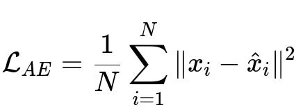
Here:

• N is the total number of training samples.

• x_i is the input vector of dimension d for the i-th training sample.

• \hat{x}_i is the reconstructed vector of dimension d from the autoencoder.

• The autoencoder’s parameters (in both encoder and decoder) are learned by minimizing this reconstruction error.

Encoder as Feature Generator

During training, the encoder learns to capture key information in the lower-dimensional bottleneck. After training:

• We can discard the decoder, keep only the encoder part, and use it to transform any new input x into the latent feature representation h.

• These h features are often more robust, denoised, and can serve as an input to other machine learning models (e.g., logistic regression, random forests, or more neural layers for various tasks).

Practical Implementation

Below is a simple PyTorch code snippet illustrating how to implement an autoencoder and generate new features from its latent layer.

import torch
import torch.nn as nn
import torch.optim as optim

# Example autoencoder
class SimpleAutoencoder(nn.Module):
    def __init__(self, input_dim=784, hidden_dim=64):
        super(SimpleAutoencoder, self).__init__()
        # Encoder
        self.encoder = nn.Sequential(
            nn.Linear(input_dim, 128),
            nn.ReLU(),
            nn.Linear(128, hidden_dim),
            nn.ReLU()
        )
        # Decoder
        self.decoder = nn.Sequential(
            nn.Linear(hidden_dim, 128),
            nn.ReLU(),
            nn.Linear(128, input_dim),
            nn.Sigmoid()
        )

    def forward(self, x):
        # x is assumed to be (batch_size, input_dim)
        encoded = self.encoder(x)
        decoded = self.decoder(encoded)
        return decoded

# Sample usage
autoencoder = SimpleAutoencoder(input_dim=784, hidden_dim=64)
criterion = nn.MSELoss()
optimizer = optim.Adam(autoencoder.parameters(), lr=1e-3)

# Suppose we have a DataLoader called train_loader giving (batch_x, _) with batch_x of shape (batch_size, 784)
# A typical training loop might look like this
for epoch in range(5):
    for batch_x, _ in train_loader:
        optimizer.zero_grad()
        reconstruction = autoencoder(batch_x)
        loss = criterion(reconstruction, batch_x)
        loss.backward()
        optimizer.step()

# Once training is done, we can generate features using the encoder
with torch.no_grad():
    for batch_x, _ in train_loader:
        features = autoencoder.encoder(batch_x)  # This is the feature vector in the bottleneck
        # features can now be used in other ML models

In this example:

• The encoder compresses the 784-dimensional input (like flattened 28x28 MNIST images) to a 64-dimensional vector.

• The decoder reconstructs the original input from the 64-dimensional latent space.

• After training, autoencoder.encoder(batch_x) gives us the new feature representation of the data.

Why Autoencoders Are Effective for Feature Generation

Autoencoders learn a data-driven compression scheme tailored to the training distribution:

• They can learn nonlinear embeddings that capture complex structures in data better than linear methods like PCA.

• They can denoise or remove irrelevant parts of the input if the architecture and regularization encourage robust encoding.

• They can incorporate domain-specific architectural innovations, such as convolutional encoders for image data, to learn features resembling those extracted by modern deep learning networks.

Follow-Up Questions

How do we choose the dimensionality of the latent space?

A common approach is to start with a dimensionality smaller than the input to ensure compression. The choice is usually guided by experimentation and domain knowledge. A too-small latent dimension can lead to under-representation (loss of essential information). A too-large dimension might fail to force the model to learn a compact, meaningful representation and can lead to overfitting or simply replicate the identity function.

What are some pitfalls when using autoencoder features?

One pitfall is overfitting, where the autoencoder simply memorizes the data without learning a useful compression. This can happen if the network is too large or not properly regularized (e.g., with dropout or weight decay). Another issue is the interpretability of the features: although the autoencoder provides features, they are not necessarily interpretable. Furthermore, if the input distribution at inference differs significantly from the training distribution, the learned features may not generalize well.

How do autoencoder-based features compare to other feature extraction methods?

Compared to handcrafted features, autoencoder features can adaptively learn from the data and potentially capture domain-specific patterns without explicit human engineering. Compared to linear methods like PCA, autoencoders can capture non-linear correlations. However, autoencoders require more data and computational resources to train, and they can be trickier to tune (e.g., choosing network architecture, regularization, and hyperparameters).

Could we use a pre-trained autoencoder from a different domain?

In some cases, a large autoencoder pre-trained on a huge dataset can be adapted to a new domain via fine-tuning, similar to transfer learning strategies used in vision or language tasks. However, significant domain shifts might require collecting representative data and training a new or partially fine-tuned model, because the latent structure learned from one domain does not always cleanly transfer to a very different domain.

Is there a difference between an autoencoder and a variational autoencoder in the context of feature generation?

A Variational Autoencoder (VAE) imposes a probabilistic framework that encourages the latent space to follow a known distribution, often a multivariate Gaussian. This leads to smoother and more continuous latent manifolds, which can be advantageous for generative tasks and controlled sampling. In standard autoencoders, the latent features may not be as smoothly distributed. However, for many downstream tasks where a stable, learned representation is needed, either approach can serve as a strong feature generator depending on the data and objectives.

Below are additional follow-up questions

1. How can autoencoders handle high-dimensional data effectively, especially when the number of features is extremely large?

Autoencoders, by design, can learn compact representations even when the input dimensionality is huge. However, several considerations apply when dealing with very high-dimensional data:

1. Architectural Depth and Width

   • Depth: Incorporating multiple layers often helps the autoencoder progressively extract hierarchical features. Deeper architectures can capture complex relationships in high-dimensional input spaces more effectively than shallow networks, provided there is sufficient training data and proper regularization.

   • Width: At each layer, sufficient capacity is needed to capture critical information. If the network is too small, it might fail to learn meaningful representations; if too large, it might overfit.

2. Regularization Strategies

   • Weight Decay (L2 Regularization): Encourages simpler weight structures, helping reduce overfitting when handling large feature sets.

   • Dropout: Randomly drops units during training, forcing more robust encodings. Especially helpful in high dimensions where certain features might dominate if left unchecked.

3. Dimensionality of the Latent Space

   • Incremental Reduction: Instead of jumping to a very small bottleneck immediately, some practitioners gradually reduce dimensions across multiple encoder layers. This step-by-step approach can help avoid abrupt loss of important information in large feature spaces.

4. Data Preprocessing

   • Scaling/Normalization: Ensures that each feature contributes proportionately, preventing certain features with large ranges from overshadowing others.

   • Sparsity: If the data is sparse, specialized techniques like sparse autoencoders can help preserve structural information.

5. Computational Considerations

   • GPU/TPU Acceleration: High-dimensional data can be computationally expensive. Hardware acceleration and efficient batching can mitigate performance bottlenecks.

   • Mini-Batch Size: Choosing appropriate batch sizes can balance memory usage with stable gradient estimates.

Subtle Pitfall

• “Curse of Dimensionality”: As dimensionality grows, distance metrics and density estimates can become less reliable. Even though autoencoders can reduce dimensionality, if the original feature space is too large without enough data samples, it’s easy for the model to overfit or to learn spurious correlations.

2. How can we incorporate domain-specific knowledge or constraints into an autoencoder architecture for improved feature generation?

In many cases, purely data-driven approaches might overlook critical domain-specific structures. There are several techniques to embed domain knowledge:

1. Custom Network Layers/Blocks

   • In specific domains (e.g., signal processing, text, images), certain operations are known to be beneficial. For instance, in audio processing, 1D convolutional layers can capture temporal dynamics. In images, 2D convolutions preserve local spatial structure.

2. Constraint-Based Loss Functions

   • Soft Constraints: Additional penalty terms (like enforcing smoothness or enforcing certain relationships between features) in the loss function can guide the network to learn physically plausible features.

   • Hard Constraints: Sometimes certain features must obey known equations (e.g., in engineering or physics contexts). Custom layers that enforce these relationships can maintain validity of the learned representation.

3. Preprocessing with Domain Heuristics

   • Before passing data to the autoencoder, transformations reflecting known domain insights can simplify learning. For instance, using log transforms in financial data if relationships are multiplicative.

4. Layer Weight Initialization

   • Initialize certain layers using prior known solutions or domain-specific patterns, so the network starts from a more informed baseline rather than random initialization.

5. Selective Encoding

   • If certain inputs are known to be correlated or hold special importance, the encoder architecture can be designed to process them together or at different scales.

Subtle Pitfall

• Over-Constraining: Embedding too many or overly strict domain constraints might prevent the model from discovering novel or unexpected patterns. Balancing domain knowledge with model flexibility is key.

3. What role does the activation function play in the encoding process, and how might different choices affect the learned features?

Activation functions introduce non-linearity, which is critical in helping an autoencoder capture complex relationships. Different activation functions can have nuanced effects:

1. Common Activations

   • ReLU (Rectified Linear Unit): Often a go-to for many deep learning applications due to simplicity and reduced vanishing gradient issues. However, ReLUs can “die” if they get stuck at negative inputs consistently.

   • Sigmoid: Bounded between [0, 1], making sense for data that is also bounded (like pixel intensities). But sigmoids can saturate, causing slow learning when inputs fall into the flat regions of the curve.

   • Tanh: Bounded between [-1, 1], often used to center data around zero. Tends to help gradient flow slightly better than sigmoids, but can still suffer from saturation.

2. Feature Sparsity vs. Smoothness

   • Certain activations (e.g., ReLU variants) naturally induce sparse representations, potentially beneficial for some tasks. Others (e.g., ELU, Leaky ReLU) can provide smoother transitions, reducing dead neurons.

3. Information Bottleneck Behavior

   • If the bottleneck layer uses an activation that excessively restricts the range (such as a sigmoid in a very low-dimensional latent space), the model might lose critical information. Conversely, using an unbounded activation might allow too much freedom, potentially leading to more training instability.

4. Experimentation

   • Choosing an activation is often empirical. The best approach is to systematically try different activations while monitoring not just reconstruction loss but also how well the features work for downstream tasks.

Subtle Pitfall

• Mismatch with Output Activation: If the final decoder uses a sigmoid activation to output data in [0,1], but the input domain isn’t actually bounded in that range, the network might learn suboptimal features. Ensuring consistency across encoder/decoder structures is crucial.

4. Are there any recommended practices for monitoring training stability in autoencoders, and how do we address training collapse or degenerate solutions?

Autoencoders can sometimes encounter degenerate solutions (e.g., the network outputting constant values) or training collapse. Strategies to monitor and mitigate these issues:

1. Validation Reconstruction Loss

   • Track reconstruction loss on a separate validation set. If the validation loss diverges while the training loss decreases, it’s a sign of overfitting. If both losses approach a constant with little variability, the network might be collapsing.

2. Latent Space Visualization

   • Occasionally sample latent vectors for random inputs and plot them. If all points collapse to a small region in latent space, the model might not be learning diverse representations.

3. Learning Rate Scheduling

   • If the learning rate is too high, gradients can explode or cause unstable oscillations. If too low, training might be too slow or get stuck. Dynamically reducing the learning rate when the validation loss plateaus can help avoid collapse.

4. Batch Normalization or Layer Normalization

   • Normalizing layer outputs can stabilize gradients and prevent the network from locking into degenerate local minima.

5. Regularly Inspect Outputs

   • Visually inspect reconstructed samples for patterns like uniform outputs or extremely noisy outputs. This quick heuristic often catches pathological behaviors early.

Subtle Pitfall

• Improper Initialization: If weights are poorly initialized, early layers might saturate or produce near-zero outputs leading to collapse. Even advanced optimizers can struggle in these scenarios.

5. How can we evaluate the quality of autoencoder-generated features beyond reconstruction error?

While reconstruction error is the most straightforward metric, it doesn’t always capture the full value of the learned features. Some additional strategies:

1. Downstream Task Performance

   • Classification/Regression Accuracy: Use the encoded features as inputs to a classifier or regressor. Compare performance against raw features or features from other dimensionality reduction techniques.

   • Clustering Metrics: If the goal is to discover inherent structure, apply clustering on latent features and evaluate with metrics like silhouette score or adjusted Rand index.

2. Visual Inspection/Embeddings

   • t-SNE or UMAP: Project the latent vectors into 2D or 3D space to see if meaningful clusters or separations appear in the embedded features. This gives insight into whether the autoencoder organizes data points well.

3. Feature Disentanglement

   • In some setups (e.g., face images), check if individual dimensions in the latent space correlate with interpretable factors (such as lighting, pose, or expression). This is trickier to quantify, but it can be revealing.

4. Reconstruction Sensitivity

   • Investigate whether small perturbations in latent space lead to large or small changes in the decoded output. A stable representation might change the reconstruction smoothly, which could be beneficial for certain tasks.

Subtle Pitfall

• Overemphasis on Low Reconstruction Error: A model might memorize input data instead of learning a generically useful representation. Good reconstruction alone doesn’t guarantee the latent space is optimal for tasks like classification or clustering.

6. In what scenarios would a convolutional autoencoder be more advantageous, and how do we adapt it to non-image data?

Convolutional autoencoders (CAEs) are specialized for preserving local structures:

1. Typical Use Cases

   • Images: Local connectivity through convolutional filters helps model spatial hierarchies effectively.

   • Videos: 3D convolutions can capture spatiotemporal features when dealing with time sequences of images.

2. Advantages

   • Parameter Efficiency: Convolutions reuse filter weights across the image, making them more efficient than fully connected layers for image-like data.

   • Preservation of Locality: Nearby pixels (or values) are processed together, aligning with how many real-world signals or images carry information in local neighborhoods.

3. Non-Image Data

   • Time Series: 1D convolutions can capture local temporal correlations (e.g., in sensor data or audio signals).

   • Graph Data: Graph convolutional networks can be adapted to handle relational structures, although they are more specialized than standard CAEs.

   • Volumetric Data: 3D convolutions can handle volumetric medical images (e.g., MRI or CT scans).

4. Architecture Adjustments

   • For non-2D data, adapt convolutional layers to the dimensionality of the input (1D for sequences, 3D for volumetric data).

   • Adjust the stride, kernel size, and padding to reflect how important local context is in the specific domain.

Subtle Pitfall

• Loss of Global Context: Purely convolutional operations focus on local receptive fields. If global relationships are essential, additional fully connected layers or global pooling mechanisms might be needed to integrate broader context.

7. What is the difference between a denoising autoencoder and a standard autoencoder in terms of feature generation, and which scenarios might favor one over the other?

Denoising autoencoders (DAEs) are trained to reconstruct clean inputs from noisy or corrupted versions, whereas standard autoencoders typically receive a clean input and attempt to reconstruct it directly:

1. Training Mechanism

   • Standard Autoencoder: Minimizes the error between the input and the reconstruction of the same input.

   • Denoising Autoencoder: Intentionally corrupts the input (e.g., by adding Gaussian noise or randomly zeroing out some inputs) before feeding it to the network, which then learns to output the uncorrupted original.

2. Feature Robustness

   • DAE: The latent representation tends to be more robust to noise because the network explicitly learns to ignore irrelevant perturbations.

   • Standard AE: May inadvertently capture and reconstruct noise if the network’s capacity is large.

3. Use Cases

   • Denoising Tasks: DAEs are naturally suited for tasks where removing noise is essential, such as cleaning images or signals.

   • General Feature Extraction: Standard AEs can suffice when data is relatively clean or if denoising is not a primary concern.

4. Impact on Latent Representation

   • Because DAEs learn to map noisy inputs to clean reconstructions, their latent space often emphasizes stable features that consistently appear across slightly varied or corrupted versions of the data.

Subtle Pitfall

• Mismatch of Noise Type: If the corruption used during training doesn’t match the real-world noise (e.g., training with Gaussian noise but actual data has different artifacts), the learned features might not be as robust as expected.

8. How does the choice of optimizer (e.g., Adam, SGD, RMSprop) impact the representation learned by an autoencoder, and are certain optimizers more suitable for certain data types or tasks?

Optimizers can influence both the speed and the stability of training, which in turn impacts the final learned representation:

1. Convergence Speed vs. Stability

   • SGD (Stochastic Gradient Descent): Might require carefully tuned learning rates and momentum. Often slower to converge but can lead to stable minima.

   • Adam: Adapts learning rates per parameter, often converging more quickly. Particularly popular for noisy, large-scale datasets.

   • RMSprop: Similar to Adam in using adaptive learning rates, often beneficial for non-stationary objectives or tasks with widely varying feature scales.

2. Generalization Properties

   • There is ongoing debate regarding which optimizer generalizes better. Some find that pure SGD can produce simpler, more generalizable solutions, while Adam might converge to solutions that reconstruct the training data very well but risk overfitting if not regularized.

3. Task-Specific Nuances

   • Sparse or Irregular Data: Adaptive optimizers (like Adam) often handle varying gradients well.

   • Very Large Datasets: Momentum-based methods (SGD with momentum, Adam) can speed up convergence.

   • Small Datasets: Slower optimizers might help avoid rapid overfitting, but thorough regularization is usually the bigger factor.

4. Practical Approach

   • Start with Adam for convenience and speed, monitor training and validation losses, then if you encounter overfitting or poor generalization, experiment with SGD or a learning rate schedule to see if it leads to a more robust latent space.

Subtle Pitfall

• Inconsistent Batch Statistics: When using adaptive optimizers, ensure consistent batch sizes. Tiny batch sizes plus adaptive learning rates can cause erratic training curves, harming representation consistency.

9. Can autoencoder-based feature generation be combined with other dimensionality reduction or manifold learning techniques, and does that lead to synergy or redundancy?

Combining autoencoders with other techniques can either provide complementary gains or can be redundant, depending on the approach:

1. Sequential Application

   • Autoencoder -> PCA: Sometimes used to further reduce dimensionality after the autoencoder. PCA might retain the bulk of variance from the latent features while removing smaller variance components.

   • Autoencoder -> t-SNE/UMAP: Typically used for visualization, providing a more interpretable 2D/3D projection of the autoencoder’s latent space.

2. Parallel or Hybrid Models

   • Manifold Regularization: Incorporate manifold constraints (like those from locally linear embedding or isometric feature mapping) into the autoencoder’s training objective. This can ensure that local geometric relationships in the input space remain consistent in the latent space.

3. Potential Benefits

   • Diverse Perspectives: Each technique has a different assumption about data structure. By combining them, one might capture both global structure (autoencoder) and local manifold structure (manifold methods).

4. Potential Redundancy

   • If the autoencoder already captures most of the data variance and local structures, applying an additional method might offer marginal improvements and increased computational overhead.

Subtle Pitfall

• Over-Complexity: Stacking too many transformations can make the final latent space more difficult to interpret and can reduce transparency about where certain improvements (or problems) arise.

10. What is the impact of batch normalization or layer normalization within the encoder/decoder on feature quality, especially for large or small datasets?

Normalization layers can significantly influence training dynamics and, by extension, the quality of the learned latent representations:

1. Batch Normalization

   • Normalizes the activations across a mini-batch, stabilizing the distribution of inputs to subsequent layers. Particularly helpful in large-batch scenarios where the mean and variance estimates are reliable.

   • Potentially speeds up training convergence and may allow for higher learning rates without instability.

2. Layer Normalization

   • Normalizes the activations across each feature dimension for a single sample, which can be more stable for smaller batch sizes or for tasks where batch statistics are highly variable.

3. Influence on Latent Space

   • Normalization can help ensure that each neuron in the bottleneck receives inputs with a stable distribution, preventing saturation or dead activations. This often improves the consistency of the learned representations.

4. Special Considerations

   • Very Small Datasets: Batch normalization might be less effective because the batch statistics can be noisy if the batch size is tiny. Layer normalization or instance normalization might be preferable.

   • Inconsistent Batches: If the data loader produces batches of varying sizes or distributions, batch normalization might lead to unstable learning. Strategies like maintaining running averages of mean and variance can mitigate this.

Subtle Pitfall

• Over-Reliance: While normalization helps with training stability, it doesn’t always solve deeper architectural or data issues (like insufficient latent space dimensionality or missing domain constraints).